Table des matières
Front Pages
Copyright Notice
This book contains large parts that are based on the book How To Think Like a Computer Scientist --- Learning with Python 3. The following is a copy of the license of this book.
Copyright (C)  Peter Wentworth, Jeffrey Elkner, Allen B. Downey and Chris Meyers.
Permission is granted to copy, distribute and/or modify this document
under the terms of the GNU Free Documentation License, Version 1.3
or any later version published by the Free Software Foundation;
with Invariant Sections being Foreword, Preface, and Contributor List, no
Front-Cover Texts, and no Back-Cover Texts.  A copy of the license is
included in the section entitled "GNU Free Documentation License".
The required sections are provided below.
As required by the "GNU Free Documentation License", this updated book is available under the same license. The updates are Copyright (C) Kim Mens, Siegfried Nijssen, Charles Pecheur.
GNU Free Documentation License
Version 1.3, 3 November 2008
Copyright 2000, 2001, 2002, 2007, 2008 Free Software Foundation, Inc.
Everyone is permitted to copy and distribute verbatim copies of this license document, but changing it is not allowed.
0. PREAMBLE
The purpose of this License is to make a manual, textbook, or other functional and useful document "free" in the sense of freedom: to assure everyone the effective freedom to copy and redistribute it, with or without modifying it, either commercially or noncommercially. Secondarily, this License preserves for the author and publisher a way to get credit for their work, while not being considered responsible for modifications made by others.
This License is a kind of "copyleft", which means that derivative works of the document must themselves be free in the same sense. It complements the GNU General Public License, which is a copyleft license designed for free software.
We have designed this License in order to use it for manuals for free software, because free software needs free documentation: a free program should come with manuals providing the same freedoms that the software does. But this License is not limited to software manuals; it can be used for any textual work, regardless of subject matter or whether it is published as a printed book. We recommend this License principally for works whose purpose is instruction or reference.
1. APPLICABILITY AND DEFINITIONS
This License applies to any manual or other work, in any medium, that contains a notice placed by the copyright holder saying it can be distributed under the terms of this License. Such a notice grants a world-wide, royalty-free license, unlimited in duration, to use that work under the conditions stated herein. The "Document", below, refers to any such manual or work. Any member of the public is a licensee, and is addressed as "you". You accept the license if you copy, modify or distribute the work in a way requiring permission under copyright law.
A "Modified Version" of the Document means any work containing the Document or a portion of it, either copied verbatim, or with modifications and/or translated into another language.
A "Secondary Section" is a named appendix or a front-matter section of the Document that deals exclusively with the relationship of the publishers or authors of the Document to the Document's overall subject (or to related matters) and contains nothing that could fall directly within that overall subject. (Thus, if the Document is in part a textbook of mathematics, a Secondary Section may not explain any mathematics.) The relationship could be a matter of historical connection with the subject or with related matters, or of legal, commercial, philosophical, ethical or political position regarding them.
The "Invariant Sections" are certain Secondary Sections whose titles are designated, as being those of Invariant Sections, in the notice that says that the Document is released under this License. If a section does not fit the above definition of Secondary then it is not allowed to be designated as Invariant. The Document may contain zero Invariant Sections. If the Document does not identify any Invariant Sections then there are none.
The "Cover Texts" are certain short passages of text that are listed, as Front-Cover Texts or Back-Cover Texts, in the notice that says that the Document is released under this License. A Front-Cover Text may be at most 5 words, and a Back-Cover Text may be at most 25 words.
A "Transparent" copy of the Document means a machine-readable copy, represented in a format whose specification is available to the general public, that is suitable for revising the document straightforwardly with generic text editors or (for images composed of pixels) generic paint programs or (for drawings) some widely available drawing editor, and that is suitable for input to text formatters or for automatic translation to a variety of formats suitable for input to text formatters. A copy made in an otherwise Transparent file format whose markup, or absence of markup, has been arranged to thwart or discourage subsequent modification by readers is not Transparent. An image format is not Transparent if used for any substantial amount of text. A copy that is not "Transparent" is called "Opaque".
Examples of suitable formats for Transparent copies include plain ASCII without markup, Texinfo input format, LaTeX input format, SGML or XML using a publicly available DTD, and standard-conforming simple HTML, PostScript or PDF designed for human modification. Examples of transparent image formats include PNG, XCF and JPG. Opaque formats include proprietary formats that can be read and edited only by proprietary word processors, SGML or XML for which the DTD and/or processing tools are not generally available, and the machine-generated HTML, PostScript or PDF produced by some word processors for output purposes only.
The "Title Page" means, for a printed book, the title page itself, plus such following pages as are needed to hold, legibly, the material this License requires to appear in the title page. For works in formats which do not have any title page as such, "Title Page" means the text near the most prominent appearance of the work's title, preceding the beginning of the body of the text.
The "publisher" means any person or entity that distributes copies of the Document to the public.
A section "Entitled XYZ" means a named subunit of the Document whose title either is precisely XYZ or contains XYZ in parentheses following text that translates XYZ in another language. (Here XYZ stands for a specific section name mentioned below, such as "Acknowledgements", "Dedications", "Endorsements", or "History".) To "Preserve the Title" of such a section when you modify the Document means that it remains a section "Entitled XYZ" according to this definition.
The Document may include Warranty Disclaimers next to the notice which states that this License applies to the Document. These Warranty Disclaimers are considered to be included by reference in this License, but only as regards disclaiming warranties: any other implication that these Warranty Disclaimers may have is void and has no effect on the meaning of this License.
2. VERBATIM COPYING
You may copy and distribute the Document in any medium, either commercially or noncommercially, provided that this License, the copyright notices, and the license notice saying this License applies to the Document are reproduced in all copies, and that you add no other conditions whatsoever to those of this License. You may not use technical measures to obstruct or control the reading or further copying of the copies you make or distribute. However, you may accept compensation in exchange for copies. If you distribute a large enough number of copies you must also follow the conditions in section 3.
You may also lend copies, under the same conditions stated above, and you may publicly display copies.
3. COPYING IN QUANTITY
If you publish printed copies (or copies in media that commonly have printed covers) of the Document, numbering more than 100, and the Document's license notice requires Cover Texts, you must enclose the copies in covers that carry, clearly and legibly, all these Cover Texts: Front-Cover Texts on the front cover, and Back-Cover Texts on the back cover. Both covers must also clearly and legibly identify you as the publisher of these copies. The front cover must present the full title with all words of the title equally prominent and visible. You may add other material on the covers in addition. Copying with changes limited to the covers, as long as they preserve the title of the Document and satisfy these conditions, can be treated as verbatim copying in other respects.
If the required texts for either cover are too voluminous to fit legibly, you should put the first ones listed (as many as fit reasonably) on the actual cover, and continue the rest onto adjacent pages.
If you publish or distribute Opaque copies of the Document numbering more than 100, you must either include a machine-readable Transparent copy along with each Opaque copy, or state in or with each Opaque copy a computer-network location from which the general network-using public has access to download using public-standard network protocols a complete Transparent copy of the Document, free of added material. If you use the latter option, you must take reasonably prudent steps, when you begin distribution of Opaque copies in quantity, to ensure that this Transparent copy will remain thus accessible at the stated location until at least one year after the last time you distribute an Opaque copy (directly or through your agents or retailers) of that edition to the public.
It is requested, but not required, that you contact the authors of the Document well before redistributing any large number of copies, to give them a chance to provide you with an updated version of the Document.
4. MODIFICATIONS
You may copy and distribute a Modified Version of the Document under the conditions of sections 2 and 3 above, provided that you release the Modified Version under precisely this License, with the Modified Version filling the role of the Document, thus licensing distribution and modification of the Modified Version to whoever possesses a copy of it. In addition, you must do these things in the Modified Version:
- A. Use in the Title Page (and on the covers, if any) a title distinct from that of the Document, and from those of previous versions (which should, if there were any, be listed in the History section of the Document). You may use the same title as a previous version if the original publisher of that version gives permission.
- B. List on the Title Page, as authors, one or more persons or entities responsible for authorship of the modifications in the Modified Version, together with at least five of the principal authors of the Document (all of its principal authors, if it has fewer than five), unless they release you from this requirement.
- C. State on the Title page the name of the publisher of the Modified Version, as the publisher.
- D. Preserve all the copyright notices of the Document.
- E. Add an appropriate copyright notice for your modifications adjacent to the other copyright notices.
- F. Include, immediately after the copyright notices, a license notice giving the public permission to use the Modified Version under the terms of this License, in the form shown in the Addendum below.
- G. Preserve in that license notice the full lists of Invariant Sections and required Cover Texts given in the Document's license notice.
- H. Include an unaltered copy of this License.
- I. Preserve the section Entitled "History", Preserve its Title, and add to it an item stating at least the title, year, new authors, and publisher of the Modified Version as given on the Title Page. If there is no section Entitled "History" in the Document, create one stating the title, year, authors, and publisher of the Document as given on its Title Page, then add an item describing the Modified Version as stated in the previous sentence.
- J. Preserve the network location, if any, given in the Document for public access to a Transparent copy of the Document, and likewise the network locations given in the Document for previous versions it was based on. These may be placed in the "History" section. You may omit a network location for a work that was published at least four years before the Document itself, or if the original publisher of the version it refers to gives permission.
- K. For any section Entitled "Acknowledgements" or "Dedications", Preserve the Title of the section, and preserve in the section all the substance and tone of each of the contributor acknowledgements and/or dedications given therein.
- L. Preserve all the Invariant Sections of the Document, unaltered in their text and in their titles. Section numbers or the equivalent are not considered part of the section titles.
- M. Delete any section Entitled "Endorsements". Such a section may not be included in the Modified Version.
- N. Do not retitle any existing section to be Entitled "Endorsements" or to conflict in title with any Invariant Section.
- O. Preserve any Warranty Disclaimers.
If the Modified Version includes new front-matter sections or appendices that qualify as Secondary Sections and contain no material copied from the Document, you may at your option designate some or all of these sections as invariant. To do this, add their titles to the list of Invariant Sections in the Modified Version's license notice. These titles must be distinct from any other section titles.
You may add a section Entitled "Endorsements", provided it contains nothing but endorsements of your Modified Version by various parties—for example, statements of peer review or that the text has been approved by an organization as the authoritative definition of a standard.
You may add a passage of up to five words as a Front-Cover Text, and a passage of up to 25 words as a Back-Cover Text, to the end of the list of Cover Texts in the Modified Version. Only one passage of Front-Cover Text and one of Back-Cover Text may be added by (or through arrangements made by) any one entity. If the Document already includes a cover text for the same cover, previously added by you or by arrangement made by the same entity you are acting on behalf of, you may not add another; but you may replace the old one, on explicit permission from the previous publisher that added the old one.
The author(s) and publisher(s) of the Document do not by this License give permission to use their names for publicity for or to assert or imply endorsement of any Modified Version.
5. COMBINING DOCUMENTS
You may combine the Document with other documents released under this License, under the terms defined in section 4 above for modified versions, provided that you include in the combination all of the Invariant Sections of all of the original documents, unmodified, and list them all as Invariant Sections of your combined work in its license notice, and that you preserve all their Warranty Disclaimers.
The combined work need only contain one copy of this License, and multiple identical Invariant Sections may be replaced with a single copy. If there are multiple Invariant Sections with the same name but different contents, make the title of each such section unique by adding at the end of it, in parentheses, the name of the original author or publisher of that section if known, or else a unique number. Make the same adjustment to the section titles in the list of Invariant Sections in the license notice of the combined work.
In the combination, you must combine any sections Entitled "History" in the various original documents, forming one section Entitled "History"; likewise combine any sections Entitled "Acknowledgements", and any sections Entitled "Dedications". You must delete all sections Entitled "Endorsements".
6. COLLECTIONS OF DOCUMENTS
You may make a collection consisting of the Document and other documents released under this License, and replace the individual copies of this License in the various documents with a single copy that is included in the collection, provided that you follow the rules of this License for verbatim copying of each of the documents in all other respects.
You may extract a single document from such a collection, and distribute it individually under this License, provided you insert a copy of this License into the extracted document, and follow this License in all other respects regarding verbatim copying of that document.
7. AGGREGATION WITH INDEPENDENT WORKS
A compilation of the Document or its derivatives with other separate and independent documents or works, in or on a volume of a storage or distribution medium, is called an "aggregate" if the copyright resulting from the compilation is not used to limit the legal rights of the compilation's users beyond what the individual works permit. When the Document is included in an aggregate, this License does not apply to the other works in the aggregate which are not themselves derivative works of the Document.
If the Cover Text requirement of section 3 is applicable to these copies of the Document, then if the Document is less than one half of the entire aggregate, the Document's Cover Texts may be placed on covers that bracket the Document within the aggregate, or the electronic equivalent of covers if the Document is in electronic form. Otherwise they must appear on printed covers that bracket the whole aggregate.
8. TRANSLATION
Translation is considered a kind of modification, so you may distribute translations of the Document under the terms of section 4. Replacing Invariant Sections with translations requires special permission from their copyright holders, but you may include translations of some or all Invariant Sections in addition to the original versions of these Invariant Sections. You may include a translation of this License, and all the license notices in the Document, and any Warranty Disclaimers, provided that you also include the original English version of this License and the original versions of those notices and disclaimers. In case of a disagreement between the translation and the original version of this License or a notice or disclaimer, the original version will prevail.
If a section in the Document is Entitled "Acknowledgements", "Dedications", or "History", the requirement (section 4) to Preserve its Title (section 1) will typically require changing the actual title.
9. TERMINATION
You may not copy, modify, sublicense, or distribute the Document except as expressly provided under this License. Any attempt otherwise to copy, modify, sublicense, or distribute it is void, and will automatically terminate your rights under this License.
However, if you cease all violation of this License, then your license from a particular copyright holder is reinstated (a) provisionally, unless and until the copyright holder explicitly and finally terminates your license, and (b) permanently, if the copyright holder fails to notify you of the violation by some reasonable means prior to 60 days after the cessation.
Moreover, your license from a particular copyright holder is reinstated permanently if the copyright holder notifies you of the violation by some reasonable means, this is the first time you have received notice of violation of this License (for any work) from that copyright holder, and you cure the violation prior to 30 days after your receipt of the notice.
Termination of your rights under this section does not terminate the licenses of parties who have received copies or rights from you under this License. If your rights have been terminated and not permanently reinstated, receipt of a copy of some or all of the same material does not give you any rights to use it.
10. FUTURE REVISIONS OF THIS LICENSE
The Free Software Foundation may publish new, revised versions of the GNU Free Documentation License from time to time. Such new versions will be similar in spirit to the present version, but may differ in detail to address new problems or concerns. See http://www.gnu.org/copyleft/.
Each version of the License is given a distinguishing version number. If the Document specifies that a particular numbered version of this License "or any later version" applies to it, you have the option of following the terms and conditions either of that specified version or of any later version that has been published (not as a draft) by the Free Software Foundation. If the Document does not specify a version number of this License, you may choose any version ever published (not as a draft) by the Free Software Foundation. If the Document specifies that a proxy can decide which future versions of this License can be used, that proxy's public statement of acceptance of a version permanently authorizes you to choose that version for the Document.
11. RELICENSING
"Massive Multiauthor Collaboration Site" (or "MMC Site") means any World Wide Web server that publishes copyrightable works and also provides prominent facilities for anybody to edit those works. A public wiki that anybody can edit is an example of such a server. A "Massive Multiauthor Collaboration" (or "MMC") contained in the site means any set of copyrightable works thus published on the MMC site.
"CC-BY-SA" means the Creative Commons Attribution-Share Alike 3.0 license published by Creative Commons Corporation, a not-for-profit corporation with a principal place of business in San Francisco, California, as well as future copyleft versions of that license published by that same organization.
"Incorporate" means to publish or republish a Document, in whole or in part, as part of another Document.
An MMC is "eligible for relicensing" if it is licensed under this License, and if all works that were first published under this License somewhere other than this MMC, and subsequently incorporated in whole or in part into the MMC, (1) had no cover texts or invariant sections, and (2) were thus incorporated prior to November 1, 2008.
The operator of an MMC Site may republish an MMC contained in the site under CC-BY-SA on the same site at any time before August 1, 2009, provided the MMC is eligible for relicensing.
ADDENDUM: How to use this License for your documents
To use this License in a document you have written, include a copy of the License in the document and put the following copyright and license notices just after the title page:
Copyright (C)  YEAR  YOUR NAME.
Permission is granted to copy, distribute and/or modify this document
under the terms of the GNU Free Documentation License, Version 1.3
or any later version published by the Free Software Foundation;
with no Invariant Sections, no Front-Cover Texts, and no Back-Cover Texts.
A copy of the license is included in the section entitled "GNU
Free Documentation License".
If you have Invariant Sections, Front-Cover Texts and Back-Cover Texts, replace the "with … Texts." line with this:
with the Invariant Sections being LIST THEIR TITLES, with the
Front-Cover Texts being LIST, and with the Back-Cover Texts being LIST.
If you have Invariant Sections without Cover Texts, or some other combination of the three, merge those two alternatives to suit the situation.
If your document contains nontrivial examples of program code, we recommend releasing these examples in parallel under your choice of free software license, such as the GNU General Public License, to permit their use in free software.
Foreword
This the foreword of "How To Think Like a Computer Scientist --- Learning with Python 3"
By David Beazley
As an educator, researcher, and book author, I am delighted to see the completion of this book. Python is a fun and extremely easy-to-use programming language that has steadily gained in popularity over the last few years. Developed over ten years ago by Guido van Rossum, Python's simple syntax and overall feel is largely derived from ABC, a teaching language that was developed in the 1980's. However, Python was also created to solve real problems and it borrows a wide variety of features from programming languages such as C++, Java, Modula-3, and Scheme. Because of this, one of Python's most remarkable features is its broad appeal to professional software developers, scientists, researchers, artists, and educators.
Despite Python's appeal to many different communities, you may still wonder why Python? or why teach programming with Python? Answering these questions is no simple task---especially when popular opinion is on the side of more masochistic alternatives such as C++ and Java. However, I think the most direct answer is that programming in Python is simply a lot of fun and more productive.
When I teach computer science courses, I want to cover important concepts in addition to making the material interesting and engaging to students. Unfortunately, there is a tendency for introductory programming courses to focus far too much attention on mathematical abstraction and for students to become frustrated with annoying problems related to low-level details of syntax, compilation, and the enforcement of seemingly arcane rules. Although such abstraction and formalism is important to professional software engineers and students who plan to continue their study of computer science, taking such an approach in an introductory course mostly succeeds in making computer science boring. When I teach a course, I don't want to have a room of uninspired students. I would much rather see them trying to solve interesting problems by exploring different ideas, taking unconventional approaches, breaking the rules, and learning from their mistakes. In doing so, I don't want to waste half of the semester trying to sort out obscure syntax problems, unintelligible compiler error messages, or the several hundred ways that a program might generate a general protection fault.
One of the reasons why I like Python is that it provides a really nice balance between the practical and the conceptual. Since Python is interpreted, beginners can pick up the language and start doing neat things almost immediately without getting lost in the problems of compilation and linking. Furthermore, Python comes with a large library of modules that can be used to do all sorts of tasks ranging from web-programming to graphics. Having such a practical focus is a great way to engage students and it allows them to complete significant projects. However, Python can also serve as an excellent foundation for introducing important computer science concepts. Since Python fully supports procedures and classes, students can be gradually introduced to topics such as procedural abstraction, data structures, and object-oriented programming --- all of which are applicable to later courses on Java or C++. Python even borrows a number of features from functional programming languages and can be used to introduce concepts that would be covered in more detail in courses on Scheme and Lisp.
In reading Jeffrey's preface, I am struck by his comments that Python allowed him to see a higher level of success and a lower level of frustration and that he was able to move faster with better results. Although these comments refer to his introductory course, I sometimes use Python for these exact same reasons in advanced graduate level computer science courses at the University of Chicago. In these courses, I am constantly faced with the daunting task of covering a lot of difficult course material in a blistering nine week quarter. Although it is certainly possible for me to inflict a lot of pain and suffering by using a language like C++, I have often found this approach to be counterproductive---especially when the course is about a topic unrelated to just programming. I find that using Python allows me to better focus on the actual topic at hand while allowing students to complete substantial class projects.
Although Python is still a young and evolving language, I believe that it has a bright future in education. This book is an important step in that direction. David Beazley University of Chicago Author of the Python Essential Reference
Contributor List
This is the contributor list of "How To Think Like a Computer Scientist --- Learning with Python 3"
To paraphrase the philosophy of the Free Software Foundation, this book is free like free speech, but not necessarily free like free pizza. It came about because of a collaboration that would not have been possible without the GNU Free Documentation License. So we would like to thank the Free Software Foundation for developing this license and, of course, making it available to us.
We would also like to thank the more than 100 sharp-eyed and thoughtful readers who have sent us suggestions and corrections over the past few years. In the spirit of free software, we decided to express our gratitude in the form of a contributor list. Unfortunately, this list is not complete, but we are doing our best to keep it up to date. It was also getting too large to include everyone who sends in a typo or two. You have our gratitude, and you have the personal satisfaction of making a book you found useful better for you and everyone else who uses it. New additions to the list for the 2nd edition will be those who have made on-going contributions.
If you have a chance to look through the list, you should realize that each person here has spared you and all subsequent readers from the confusion of a technical error or a less-than-transparent explanation, just by sending us a note.
Impossible as it may seem after so many corrections, there may still be errors in this book. If you should stumble across one, we hope you will take a minute to contact us. The email address (for the Python 3 version of the book) is p.wentworth@ru.ac.za . Substantial changes made due to your suggestions will add you to the next version of the contributor list (unless you ask to be omitted). Thank you!
Second Edition
- An email from Mike MacHenry set me straight on tail recursion. He not only pointed out an error in the presentation, but suggested how to correct it.
- It wasn't until 5th Grade student Owen Davies came to me in a Saturday morning Python enrichment class and said he wanted to write the card game, Gin Rummy, in Python that I finally knew what I wanted to use as the case study for the object oriented programming chapters.
- A special thanks to pioneering students in Jeff's Python Programming class at GCTAA during the 2009-2010 school year: Safath Ahmed, Howard Batiste, Louis Elkner-Alfaro, and Rachel Hancock. Your continual and thoughtfull feedback led to changes in most of the chapters of the book. You set the standard for the active and engaged learners that will help make the new Governor's Academy what it is to become. Thanks to you this is truly a student tested text.
- Thanks in a similar vein to the students in Jeff's Computer Science class at the HB-Woodlawn program during the 2007-2008 school year: James Crowley, Joshua Eddy, Eric Larson, Brian McGrail, and Iliana Vazuka.
- Ammar Nabulsi sent in numerous corrections from Chapters 1 and 2.
- Aldric Giacomoni pointed out an error in our definition of the Fibonacci sequence in Chapter 5.
- Roger Sperberg sent in several spelling corrections and pointed out a twisted piece of logic in Chapter 3.
- Adele Goldberg sat down with Jeff at PyCon 2007 and gave him a list of suggestions and corrections from throughout the book.
- Ben Bruno sent in corrections for chapters 4, 5, 6, and 7.
- Carl LaCombe pointed out that we incorrectly used the term commutative in chapter 6 where symmetric was the correct term.
- Alessandro Montanile sent in corrections for errors in the code examples and text in chapters 3, 12, 15, 17, 18, 19, and 20.
- Emanuele Rusconi found errors in chapters 4, 8, and 15.
- Michael Vogt reported an indentation error in an example in chapter 6, and sent in a suggestion for improving the clarity of the shell vs. script section in chapter 1.
First Edition
- Lloyd Hugh Allen sent in a correction to Section 8.4.
- Yvon Boulianne sent in a correction of a semantic error in Chapter 5.
- Fred Bremmer submitted a correction in Section 2.1.
- Jonah Cohen wrote the Perl scripts to convert the LaTeX source for this book into beautiful HTML.
- Michael Conlon sent in a grammar correction in Chapter 2 and an improvement in style in Chapter 1, and he initiated discussion on the technical aspects of interpreters.
- Benoit Girard sent in a correction to a humorous mistake in Section 5.6.
- Courtney Gleason and Katherine Smith wrote horsebet.py, which was used as a case study in an earlier version of the book. Their program can now be found on the website.
- Lee Harr submitted more corrections than we have room to list here, and indeed he should be listed as one of the principal editors of the text.
- James Kaylin is a student using the text. He has submitted numerous corrections.
- David Kershaw fixed the broken catTwice function in Section 3.10.
- Eddie Lam has sent in numerous corrections to Chapters 1, 2, and 3. He also fixed the Makefile so that it creates an index the first time it is run and helped us set up a versioning scheme.
- Man-Yong Lee sent in a correction to the example code in Section 2.4.
- David Mayo pointed out that the word unconsciously in Chapter 1 needed to be changed to subconsciously .
- Chris McAloon sent in several corrections to Sections 3.9 and 3.10.
- Matthew J. Moelter has been a long-time contributor who sent in numerous corrections and suggestions to the book.
- Simon Dicon Montford reported a missing function definition and several typos in Chapter 3. He also found errors in the increment function in Chapter 13.
- John Ouzts corrected the definition of return value in Chapter 3.
- Kevin Parks sent in valuable comments and suggestions as to how to improve the distribution of the book.
- David Pool sent in a typo in the glossary of Chapter 1, as well as kind words of encouragement.
- Michael Schmitt sent in a correction to the chapter on files and exceptions.
- Robin Shaw pointed out an error in Section 13.1, where the printTime function was used in an example without being defined.
- Paul Sleigh found an error in Chapter 7 and a bug in Jonah Cohen's Perl script that generates HTML from LaTeX.
- Craig T. Snydal is testing the text in a course at Drew University. He has contributed several valuable suggestions and corrections.
- Ian Thomas and his students are using the text in a programming course. They are the first ones to test the chapters in the latter half of the book, and they have make numerous corrections and suggestions.
- Keith Verheyden sent in a correction in Chapter 3.
- Peter Winstanley let us know about a longstanding error in our Latin in Chapter 3.
- Chris Wrobel made corrections to the code in the chapter on file I/O and exceptions.
- Moshe Zadka has made invaluable contributions to this project. In addition to writing the first draft of the chapter on Dictionaries, he provided continual guidance in the early stages of the book.
- Christoph Zwerschke sent several corrections and pedagogic suggestions, and explained the difference between gleich and selbe.
- James Mayer sent us a whole slew of spelling and typographical errors, including two in the contributor list.
- Hayden McAfee caught a potentially confusing inconsistency between two examples.
- Angel Arnal is part of an international team of translators working on the Spanish version of the text. He has also found several errors in the English version.
- Tauhidul Hoque and Lex Berezhny created the illustrations in Chapter 1 and improved many of the other illustrations.
- Dr. Michele Alzetta caught an error in Chapter 8 and sent some interesting pedagogic comments and suggestions about Fibonacci and Old Maid.
- Andy Mitchell caught a typo in Chapter 1 and a broken example in Chapter 2.
- Kalin Harvey suggested a clarification in Chapter 7 and caught some typos.
- Christopher P. Smith caught several typos and is helping us prepare to update the book for Python 2.2.
- David Hutchins caught a typo in the Foreword.
- Gregor Lingl is teaching Python at a high school in Vienna, Austria. He is working on a German translation of the book, and he caught a couple of bad errors in Chapter 5.
- Julie Peters caught a typo in the Preface.
Preface
This the preface of "How To Think Like a Computer Scientist --- Learning with Python 3"
By Jeffrey Elkner
This book owes its existence to the collaboration made possible by the Internet and the free software movement. Its three authors---a college professor, a high school teacher, and a professional programmer---never met face to face to work on it, but we have been able to collaborate closely, aided by many other folks who have taken the time and energy to send us their feedback.
We think this book is a testament to the benefits and future possibilities of this kind of collaboration, the framework for which has been put in place by Richard Stallman and the Free Software Foundation.
How and why I came to use Python
In 1999, the College Board's Advanced Placement (AP) Computer Science exam was given in C++ for the first time. As in many high schools throughout the country, the decision to change languages had a direct impact on the computer science curriculum at Yorktown High School in Arlington, Virginia, where I teach. Up to this point, Pascal was the language of instruction in both our first-year and AP courses. In keeping with past practice of giving students two years of exposure to the same language, we made the decision to switch to C++ in the first year course for the 1997-98 school year so that we would be in step with the College Board's change for the AP course the following year.
Two years later, I was convinced that C++ was a poor choice to use for introducing students to computer science. While it is certainly a very powerful programming language, it is also an extremely difficult language to learn and teach. I found myself constantly fighting with C++'s difficult syntax and multiple ways of doing things, and I was losing many students unnecessarily as a result. Convinced there had to be a better language choice for our first-year class, I went looking for an alternative to C++.
I needed a language that would run on the machines in our GNU/Linux lab as well as on the Windows and Macintosh platforms most students have at home. I wanted it to be free software, so that students could use it at home regardless of their income. I wanted a language that was used by professional programmers, and one that had an active developer community around it. It had to support both procedural and object-oriented programming. And most importantly, it had to be easy to learn and teach. When I investigated the choices with these goals in mind, Python stood out as the best candidate for the job.
I asked one of Yorktown's talented students, Matt Ahrens, to give Python a try. In two months he not only learned the language but wrote an application called pyTicket that enabled our staff to report technology problems via the Web. I knew that Matt could not have finished an application of that scale in so short a time in C++, and this accomplishment, combined with Matt's positive assessment of Python, suggested that Python was the solution I was looking for.
Finding a textbook
Having decided to use Python in both of my introductory computer science classes the following year, the most pressing problem was the lack of an available textbook.
Free documents came to the rescue. Earlier in the year, Richard Stallman had introduced me to Allen Downey. Both of us had written to Richard expressing an interest in developing free educational materials. Allen had already written a first-year computer science textbook, How to Think Like a Computer Scientist. When I read this book, I knew immediately that I wanted to use it in my class. It was the clearest and most helpful computer science text I had seen. It emphasized the processes of thought involved in programming rather than the features of a particular language. Reading it immediately made me a better teacher.
How to Think Like a Computer Scientist was not just an excellent book, but it had been released under the GNU public license, which meant it could be used freely and modified to meet the needs of its user. Once I decided to use Python, it occurred to me that I could translate Allen's original Java version of the book into the new language. While I would not have been able to write a textbook on my own, having Allen's book to work from made it possible for me to do so, at the same time demonstrating that the cooperative development model used so well in software could also work for educational materials.
Working on this book for the last two years has been rewarding for both my students and me, and my students played a big part in the process. Since I could make instant changes whenever someone found a spelling error or difficult passage, I encouraged them to look for mistakes in the book by giving them a bonus point each time they made a suggestion that resulted in a change in the text. This had the double benefit of encouraging them to read the text more carefully and of getting the text thoroughly reviewed by its most important critics, students using it to learn computer science.
For the second half of the book on object-oriented programming, I knew that someone with more real programming experience than I had would be needed to do it right. The book sat in an unfinished state for the better part of a year until the open source community once again provided the needed means for its completion.
I received an email from Chris Meyers expressing interest in the book. Chris is a professional programmer who started teaching a programming course last year using Python at Lane Community College in Eugene, Oregon. The prospect of teaching the course had led Chris to the book, and he started helping out with it immediately. By the end of the school year he had created a companion project on our Website at http://openbookproject.net called *Python for Fun* and was working with some of my most advanced students as a master teacher, guiding them beyond where I could take them.
Introducing programming with Python
The process of translating and using How to Think Like a Computer Scientist for the past two years has confirmed Python's suitability for teaching beginning students. Python greatly simplifies programming examples and makes important programming ideas easier to teach.
The first example from the text illustrates this point. It is the traditional hello, world program, which in the Java version of the book looks like this:
class Hello {

  public static void main (String[] args) {
      System.out.println ("Hello, world.");
  }
}
in the Python version it becomes:
print("Hello, World!")
Even though this is a trivial example, the advantages of Python stand out. Yorktown's Computer Science I course has no prerequisites, so many of the students seeing this example are looking at their first program. Some of them are undoubtedly a little nervous, having heard that computer programming is difficult to learn. The Java version has always forced me to choose between two unsatisfying options: either to explain the class Hello, public static void main, String[] args, {, and }, statements and risk confusing or intimidating some of the students right at the start, or to tell them, Just don't worry about all of that stuff now; we will talk about it later, and risk the same thing. The educational objectives at this point in the course are to introduce students to the idea of a programming statement and to get them to write their first program, thereby introducing them to the programming environment. The Python program has exactly what is needed to do these things, and nothing more.
Comparing the explanatory text of the program in each version of the book further illustrates what this means to the beginning student. There are seven paragraphs of explanation of Hello, world! in the Java version; in the Python version, there are only a few sentences. More importantly, the missing six paragraphs do not deal with the big ideas in computer programming but with the minutia of Java syntax. I found this same thing happening throughout the book. Whole paragraphs simply disappear from the Python version of the text because Python's much clearer syntax renders them unnecessary.
Using a very high-level language like Python allows a teacher to postpone talking about low-level details of the machine until students have the background that they need to better make sense of the details. It thus creates the ability to put first things first pedagogically. One of the best examples of this is the way in which Python handles variables. In Java a variable is a name for a place that holds a value if it is a built-in type, and a reference to an object if it is not. Explaining this distinction requires a discussion of how the computer stores data. Thus, the idea of a variable is bound up with the hardware of the machine. The powerful and fundamental concept of a variable is already difficult enough for beginning students (in both computer science and algebra). Bytes and addresses do not help the matter. In Python a variable is a name that refers to a thing. This is a far more intuitive concept for beginning students and is much closer to the meaning of variable that they learned in their math courses. I had much less difficulty teaching variables this year than I did in the past, and I spent less time helping students with problems using them.
Another example of how Python aids in the teaching and learning of programming is in its syntax for functions. My students have always had a great deal of difficulty understanding functions. The main problem centers around the difference between a function definition and a function call, and the related distinction between a parameter and an argument. Python comes to the rescue with syntax that is nothing short of beautiful. Function definitions begin with the keyword def, so I simply tell my students, When you define a function, begin with def, followed by the name of the function that you are defining; when you call a function, simply call (type) out its name. Parameters go with definitions; arguments go with calls. There are no return types, parameter types, or reference and value parameters to get in the way, so I am now able to teach functions in less than half the time that it previously took me, with better comprehension.
Using Python improved the effectiveness of our computer science program for all students. I saw a higher general level of success and a lower level of frustration than I experienced teaching with either C++ or Java. I moved faster with better results. More students left the course with the ability to create meaningful programs and with the positive attitude toward the experience of programming that this engenders.
Building a community
I have received email from all over the globe from people using this book to learn or to teach programming. A user community has begun to emerge, and many people have been contributing to the project by sending in materials for the companion Website at http://openbookproject.net/pybiblio.
With the continued growth of Python, I expect the growth in the user community to continue and accelerate. The emergence of this user community and the possibility it suggests for similar collaboration among educators have been the most exciting parts of working on this project for me. By working together, we can increase the quality of materials available for our use and save valuable time. I invite you to join our community and look forward to hearing from you. Please write to me at jeff@elkner.net.
Table des matières
Introduction
The way of the program
Source: this section is heavily based on Chapter 1 of [ThinkCS].
The goal of this book is to teach you to think like a computer scientist. This way of thinking combines some of the best features of mathematics, engineering, and natural science. Like mathematicians, computer scientists use formal languages to denote ideas (specifically computations). Like engineers, they design things, assembling components into systems and evaluating tradeoffs among alternatives. Like scientists, they observe the behavior of complex systems, form hypotheses, and test predictions.
The single most important skill for a computer scientist is problem solving. Problem solving means the ability to formulate problems, think creatively about solutions, and express a solution clearly and accurately. As it turns out, the process of learning to program is an excellent opportunity to practice problem-solving skills. That's why this chapter is called, The way of the program.
On one level, you will be learning to program, a useful skill by itself. On another level, you will use programming as a means to an end. As we go along, that end will become clearer.
The Python programming language
The programming language you will be learning is Python. Python is an example of a high-level language; other high-level languages you might have heard of are C++, PHP, Pascal, C#, and Java.
As you might infer from the name high-level language, there are also low-level languages, sometimes referred to as machine languages or assembly languages. Loosely speaking, computers can only execute programs written in low-level languages. Thus, programs written in a high-level language have to be translated into something more suitable before they can run.
Almost all programs are written in high-level languages because of their advantages. It is much easier to program in a high-level language so programs take less time to write, they are shorter and easier to read, and they are more likely to be correct. Second, high-level languages are portable, meaning that they can run on different kinds of computers with few or no modifications.
The engine that translates and runs Python is called the Python Interpreter: There are two ways to use it: immediate mode and script mode. In immediate mode, you type Python expressions that are executed immediately. This looks as follows:
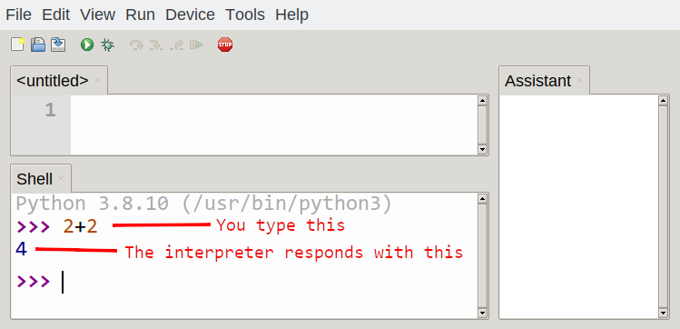
The >>> is called the Python prompt. The interpreter uses the prompt to indicate that it is ready for instructions. We typed 2 + 2, and the interpreter evaluated our expression, and replied 4, and on the next line it gave a new prompt, indicating that it is ready for more input.
Alternatively, you can write a program in a file and use the interpreter to execute the contents of the file. Such a file is called a script. Scripts have the advantage that they can be saved to disk, printed, and so on.
In this course, we use a program development environment called Thonny. (It is available at https://thonny.org.) There are various other development environments. If you're using one of the others, you might be better off working with the authors' original book rather than this edition.
For example, we created a file named firstprogram.py using Thonny. By convention, files that contain Python programs have names that end with .py.
To execute the program, we can click the Run button in Thonny:
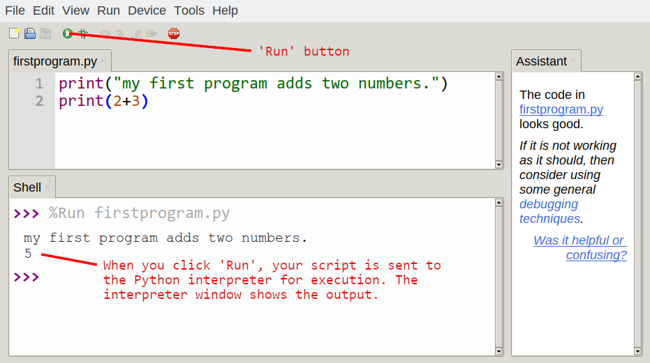
Most programs are more interesting than this one.
Working directly in the interpreter is convenient for testing short bits of code because you get immediate feedback. Think of it as scratch paper used to help you work out problems. Anything longer than a few lines should be put into a script.
What is a program?
A program is a sequence of instructions that specifies how to perform a computation. The computation might be something mathematical, such as solving a system of equations or finding the roots of a polynomial, but it can also be a symbolic computation, such as searching and replacing text in a document or (strangely enough) compiling a program.
The details look different in different languages, but a few basic instructions appear in just about every language:
- input
- Get data from the keyboard, a file, or some other device.
- output
- Display data on the screen or send data to a file or other device.
- math
- Perform basic mathematical operations like addition and multiplication.
- conditional execution
- Check for certain conditions and execute the appropriate sequence of statements.
- repetition
- Perform some action repeatedly, usually with some variation.
Believe it or not, that's pretty much all there is to it. Every program you've ever used, no matter how complicated, is made up of instructions that look more or less like these. Thus, we can describe programming as the process of breaking a large, complex task into smaller and smaller subtasks until the subtasks are simple enough to be performed with sequences of these basic instructions.
That may be a little vague, but we will come back to this topic later when we talk about algorithms.
What is debugging?
Programming is a complex process, and because it is done by human beings, it often leads to errors. Programming errors are called bugs and the process of tracking them down and correcting them is called debugging. Use of the term bug to describe small engineering difficulties dates back to at least 1889, when Thomas Edison had a bug with his phonograph.
Three kinds of errors can occur in a program: syntax errors, runtime errors, and semantic errors. It is useful to distinguish between them in order to track them down more quickly.
Syntax errors
Python can only execute a program if the program is syntactically correct; otherwise, the process fails and returns an error message. Syntax refers to the structure of a program and the rules about that structure. For example, in English, a sentence must begin with a capital letter and end with a period. this sentence contains a syntax error. So does this one
For most readers, a few syntax errors are not a significant problem, which is why we can read the poetry of E. E. Cummings without problems. Python is not so forgiving. If there is a single syntax error anywhere in your program, Python will display an error message and quit, and you will not be able to run your program. During the first few weeks of your programming career, you will probably spend a lot of time tracking down syntax errors. As you gain experience, though, you will make fewer errors and find them faster.
Runtime errors
The second type of error is a runtime error, so called because the error does not appear until you run the program. These errors are also called exceptions because they usually indicate that something exceptional (and bad) has happened.
Runtime errors are rare in the simple programs you will see in the first few chapters, so it might be a while before you encounter one.
Semantic errors
The third type of error is the semantic error. If there is a semantic error in your program, it will run successfully, in the sense that the computer will not generate any error messages, but it will not do the right thing. It will do something else. Specifically, it will do what you told it to do.
The problem is that the program you wrote is not the program you wanted to write. The meaning of the program (its semantics) is wrong. Identifying semantic errors can be tricky because it requires you to work backward by looking at the output of the program and trying to figure out what it is doing.
Experimental debugging
One of the most important skills you will acquire is debugging. Although it can be frustrating, debugging is one of the most intellectually rich, challenging, and interesting parts of programming.
In some ways, debugging is like detective work. You are confronted with clues, and you have to infer the processes and events that led to the results you see.
Debugging is also like an experimental science. Once you have an idea what is going wrong, you modify your program and try again. If your hypothesis was correct, then you can predict the result of the modification, and you take a step closer to a working program. If your hypothesis was wrong, you have to come up with a new one. As Sherlock Holmes pointed out, When you have eliminated the impossible, whatever remains, however improbable, must be the truth. (A. Conan Doyle, The Sign of Four)
For some people, programming and debugging are the same thing. That is, programming is the process of gradually debugging a program until it does what you want. The idea is that you should start with a program that does something and make small modifications, debugging them as you go, so that you always have a working program.
For example, Linux is an operating system kernel that contains millions of lines of code, but it started out as a simple program Linus Torvalds used to explore the Intel 80386 chip. According to Larry Greenfield, one of Linus's earlier projects was a program that would switch between displaying AAAA and BBBB. This later evolved to Linux (The Linux Users' Guide Beta Version 1).
Later chapters will make more suggestions about debugging and other programming practices.
Formal and natural languages
Natural languages are the languages that people speak, such as English, Spanish, and French. They were not designed by people (although people try to impose some order on them); they evolved naturally.
Formal languages are languages that are designed by people for specific applications. For example, the notation that mathematicians use is a formal language that is particularly good at denoting relationships among numbers and symbols. Chemists use a formal language to represent the chemical structure of molecules. And most importantly:
Programming languages are formal languages that have been designed to express computations.
Formal languages tend to have strict rules about syntax. For example, 3+3=6 is a syntactically correct mathematical statement, but 3=+6$ is not. H2O is a syntactically correct chemical name, but 2Zz is not.
Syntax rules come in two flavors, pertaining to tokens and structure. Tokens are the basic elements of the language, such as words, numbers, parentheses, commas, and so on. In Python, a statement like print("Happy New Year for ",2013) has 6 tokens: a function name, an open parenthesis (round bracket), a string, a comma, a number, and a close parenthesis.
It is possible to make errors in the way one constructs tokens. One of the problems with 3=+6$ is that $ is not a legal token in mathematics (at least as far as we know). Similarly, 2Zz is not a legal token in chemistry notation because there is no element with the abbreviation Zz.
The second type of syntax rule pertains to the structure of a statement--- that is, the way the tokens are arranged. The statement 3=+6$ is structurally illegal because you can't place a plus sign immediately after an equal sign. Similarly, molecular formulas have to have subscripts after the element name, not before. And in our Python example, if we omitted the comma, or if we changed the two parentheses around to say print)"Happy New Year for ",2013( our statement would still have six legal and valid tokens, but the structure is illegal.
When you read a sentence in English or a statement in a formal language, you have to figure out what the structure of the sentence is (although in a natural language you do this subconsciously). This process is called parsing.
For example, when you hear the sentence, "The other shoe fell", you understand that the other shoe is the subject and fell is the verb. Once you have parsed a sentence, you can figure out what it means, or the semantics of the sentence. Assuming that you know what a shoe is and what it means to fall, you will understand the general implication of this sentence.
Although formal and natural languages have many features in common --- tokens, structure, syntax, and semantics --- there are many differences:
- ambiguity
- Natural languages are full of ambiguity, which people deal with by using contextual clues and other information. Formal languages are designed to be nearly or completely unambiguous, which means that any statement has exactly one meaning, regardless of context.
- redundancy
- In order to make up for ambiguity and reduce misunderstandings, natural languages employ lots of redundancy. As a result, they are often verbose. Formal languages are less redundant and more concise.
- literalness
- Formal languages mean exactly what they say. On the other hand, natural languages are full of idiom and metaphor. If someone says, "The other shoe fell", there is probably no shoe and nothing falling. You'll need to find the original joke to understand the idiomatic meaning of the other shoe falling. Yahoo! Answers thinks it knows!
People who grow up speaking a natural language---everyone---often have a hard time adjusting to formal languages. In some ways, the difference between formal and natural language is like the difference between poetry and prose, but more so:
- poetry
- Words are used for their sounds as well as for their meaning, and the whole poem together creates an effect or emotional response. Ambiguity is not only common but often deliberate.
- prose
- The literal meaning of words is more important, and the structure contributes more meaning. Prose is more amenable to analysis than poetry but still often ambiguous.
- program
- The meaning of a computer program is unambiguous and literal, and can be understood entirely by analysis of the tokens and structure.
Here are some suggestions for reading programs (and other formal languages). First, remember that formal languages are much more dense than natural languages, so it takes longer to read them. Also, the structure is very important, so it is usually not a good idea to read from top to bottom, left to right. Instead, learn to parse the program in your head, identifying the tokens and interpreting the structure. Finally, the details matter. Little things like spelling errors and bad punctuation, which you can get away with in natural languages, can make a big difference in a formal language.
The first program
Traditionally, the first program written in a new language is called Hello, World! because all it does is display the words, Hello, World! In Python, the script looks like this: (For scripts, we'll show line numbers to the left of the Python statements.)
print("Hello, World!")
This is an example of using the print function, which doesn't actually print anything on paper. It displays a value on the screen. In this case, the result shown is
Hello, World!
The quotation marks in the program mark the beginning and end of the value; they don't appear in the result.
Some people judge the quality of a programming language by the simplicity of the Hello, World! program. By this standard, Python does about as well as possible.
Comments
As programs get bigger and more complicated, they get more difficult to read. Formal languages are dense, and it is often difficult to look at a piece of code and figure out what it is doing, or why.
For this reason, it is a good idea to add notes to your programs to explain in natural language what the program is doing.
A comment in a computer program is text that is intended only for the human reader --- it is completely ignored by the interpreter.
In Python, the # token starts a comment. The rest of the line is ignored. Here is a new version of Hello, World!.
#---------------------------------------------------
# This demo program shows off how elegant Python is!
# Written by Joe Soap, December 2010.
# Anyone may freely copy or modify this program.
#---------------------------------------------------

print("Hello, World!")     # Isn't this easy!
You'll also notice that we've left a blank line in the program. Blank lines are also ignored by the interpreter, but comments and blank lines can make your programs much easier for humans to parse. Use them liberally!
Glossary
- algorithm
- A set of specific steps for solving a category of problems.
- bug
- An error in a program.
- comment
- Information in a program that is meant for other programmers (or anyone reading the source code) and has no effect on the execution of the program.
- debugging
- The process of finding and removing any of the three kinds of programming errors.
- exception
- Another name for a runtime error.
- formal language
- Any one of the languages that people have designed for specific purposes, such as representing mathematical ideas or computer programs; all programming languages are formal languages.
- high-level language
- A programming language like Python that is designed to be easy for humans to read and write.
- immediate mode
- A style of using Python where we type expressions at the command prompt, and the results are shown immediately. Contrast with script, and see the entry under Python shell.
- interpreter
- The engine that executes your Python scripts or expressions.
- low-level language
- A programming language that is designed to be easy for a computer to execute; also called machine language or assembly language.
- natural language
- Any one of the languages that people speak that evolved naturally.
- object code
- The output of the compiler after it translates the program.
- parse
- To examine a program and analyze the syntactic structure.
- portability
- A property of a program that can run on more than one kind of computer.
- print function
- A function used in a program or script that causes the Python interpreter to display a value on its output device.
- problem solving
- The process of formulating a problem, finding a solution, and expressing the solution.
- program
- a sequence of instructions that specifies to a computer actions and computations to be performed.
- Python shell
- An interactive user interface to the Python interpreter. The user of a Python shell types commands at the prompt (>>>), and presses the return key to send these commands immediately to the interpreter for processing. The word shell comes from Unix. In Thonny, the Interpreter Window is where we'd do the immediate mode interaction.
- runtime error
- An error that does not occur until the program has started to execute but that prevents the program from continuing.
- script
- A program stored in a file (usually one that will be interpreted).
- semantic error
- An error in a program that makes it do something other than what the programmer intended.
- semantics
- The meaning of a program.
- source code
- A program in a high-level language before being compiled.
- syntax
- The structure of a program.
- syntax error
- An error in a program that makes it impossible to parse --- and therefore impossible to interpret.
- token
- One of the basic elements of the syntactic structure of a program, analogous to a word in a natural language.
References
| [ThinkCS] | How To Think Like a Computer Scientist --- Learning with Python 3 |
Variables, expressions and statements
Source: this section is heavily based on Chapter 2 of [ThinkCS].
Executing programs in a computer
Before going into the details of Python, it is useful to consider how computers are organised and execute programs. A computer typically consists of at least the following components:
- a processor, which executes instructions in a program; examples of well-known processors are Intel Core processors, AMD Athlon processors, Qualcomm Snapdragon processors, and Apple M1 processors.
- a main memory, which stores the program and the data while the processor is executing the program; typical capacities for the main memory are nowadays between 8GB and 32GB.
- a disk drive, which stores all files available to the computer without Internet connection; in a laptop this is nowadays 256GB or more, while on a desktop 1TB is not uncommon.
- a monitor, which displays information to the user.
- a network connection, which allows to interact with the Internet.
- a keyboard and a mouse or touchpad, which allow the user to provide input to the computer.
If you use the Python interpreter, this program is initially stored on the disk drive; when you start the interpreter, it is loaded in the main memory of the computer, such that the processor can execute the interpreter.
The main memory of the computer stores everything that the processor needs to have access to in order to execute a program. This not only includes the Python interpreter, the instructions of the program that the processor is executing, but also intermediate results of a calculation; after all, in most cases the calculation that we ask a computer to do is so complex that it needs memory to maintain the intermediate steps of a calculation.
To organize its calculations well, the Python interpreter organizes the memory in a specific manner, of which we will see more details later in this syllabus. Core ideas are the following:
- Parts of the memory are given names; these names can be used to refer to that part of the memory;
- The information that is stored in a certain part of the memory, has a value, for instance 4 or 3.0, and a type: for instance, it is a text, or a number;
- To calculate information that can be stored in a part of the memory, in Python programs we write expressions;
- To decide the order in which we perform calculations, Python programs consist of statements that are put in a certain order.
In this chapter, we will discuss each of these ideas in more detail.
Values and data types
A value is one of the fundamental things --- like a letter or a number --- that a program manipulates. The values we have seen so far are 4 (the result when we added 2 + 2), and "Hello, World!".
These values are classified into different classes, or data types: 4 is an integer, and "Hello, World!" is a string, so-called because it contains a string of letters. You (and the interpreter) can identify strings because they are enclosed in quotation marks.
If you are not sure what class a value falls into, Python has a function called type which can tell you.
>>> type("Hello, World!")
<class 'str'>
>>> type(17)
<class 'int'>
Not surprisingly, strings belong to the class str and integers belong to the class int. Less obviously, numbers with a decimal point belong to a class called float, because these numbers are represented in a format called floating-point. At this stage, you can treat the words class and type interchangeably. We'll come back to a deeper understanding of what a class is in later chapters.
>>> type(3.2)
<class 'float'>
What about values like "17" and "3.2"? They look like numbers, but they are in quotation marks like strings.
>>> type("17")
<class 'str'>
>>> type("3.2")
<class 'str'>
They're strings!
Strings in Python can be enclosed in either single quotes (') or double quotes ("), or three of each (''' or """)
>>> type('This is a string.')
<class 'str'>
>>> type("And so is this.")
<class 'str'>
>>> type("""and this.""")
<class 'str'>
>>> type('''and even this...''')
<class 'str'>
Double quoted strings can contain single quotes inside them, as in "Bruce's beard", and single quoted strings can have double quotes inside them, as in 'The knights who say "Ni!"'.
Strings enclosed with three occurrences of either quote symbol are called triple quoted strings. They can contain either single or double quotes:
>>> print('''"Oh no", she exclaimed, "Ben's bike is broken!"''')
"Oh no", she exclaimed, "Ben's bike is broken!"
>>>
Triple quoted strings can even span multiple lines:
>>> message = """This message will
... span several
... lines."""
>>> print(message)
This message will
span several
lines.
>>>
Python doesn't care whether you use single or double quotes or the three-of-a-kind quotes to surround your strings: once it has parsed the text of your program or command, the way it stores the value is identical in all cases, and the surrounding quotes are not part of the value. But when the interpreter wants to display a string, it has to decide which quotes to use to make it look like a string.
>>> 'This is a string.'
'This is a string.'
>>> """And so is this."""
'And so is this.'
So the Python language designers usually chose to surround their strings by single quotes. What do think would happen if the string already contained single quotes?
When you type a large integer, you might be tempted to use commas between groups of three digits, as in 42,000. This is not a legal integer in Python, but it does mean something else, which is legal:
>>> 42000
42000
>>> 42,000
(42, 0)
Well, that's not what we expected at all! Because of the comma, Python chose to treat this as a pair of values. We'll come back to learn about pairs later. But, for the moment, remember not to put commas or spaces in your integers, no matter how big they are. Also revisit what we said in the previous chapter: formal languages are strict, the notation is concise, and even the smallest change might mean something quite different from what you intended.
Variables
One of the most powerful features of a programming language is the ability to store values in the memory of the computer. In Python this is done by manipulating variables. A variable is a name that refers to a value stored in the memory of the computer.
The assignment statement gives a value to a variable:
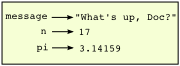
>>> message = "What's up, Doc?"
>>> n = 17
>>> pi = 3.14159
This example makes three assignments. The first assigns the string value "What's up, Doc?" to a variable named message. The second gives the integer 17 to n, and the third assigns the floating-point number 3.14159 to a variable called pi.
After executing these instructions, hence, in the memory of the computer we have three variables; each variable has a name (such as message), a type (such as str) and a value (such as "What's up, Doc?"). The assignment statement effectively changes the contents of the memory of the computer.
The assignment token, =, should not be confused with equals, which uses the token ==. The assignment statement binds a name, on the left-hand side of the operator, to a value, on the right-hand side. This is why you will get an error if you enter:
>>> 17 = n
File "<interactive input>", line 1
SyntaxError: can't assign to literal
Tip
When reading or writing code, say to yourself "n is assigned 17" or "n gets the value 17". Don't say "n equals 17".
A common way to represent variables on paper is to write the name with an arrow pointing to the variable's value. This kind of figure is called a state snapshot because it shows what state each of the variables is in at a particular instant in time. (Think of it as the variable's state of mind). This diagram shows the result of executing the assignment statements:
If you ask the interpreter to evaluate a variable, it will produce the value that is currently linked to the variable:
>>> message
"What's up, Doc?"
>>> n
17
>>> pi
3.14159
We use variables in a program to "remember" things, perhaps the current score at the football game. But variables are variable. This means they can change over time, just like the scoreboard at a football game. You can assign a value to a variable, and later assign a different value to the same variable. (This is different from maths. In maths, if you give `x` the value 3, it cannot change to link to a different value half-way through your calculations!)
>>> day = "Thursday"
>>> day
'Thursday'
>>> day = "Friday"
>>> day
'Friday'
>>> day = 21
>>> day
21
You'll notice we changed the value of day three times, and on the third assignment we even made it refer to a value that was of a different type.
A great deal of programming is about having the computer remember things, e.g. The number of missed calls on your phone, and then arranging to update or change the variable when you miss another call.
Variable names and keywords
Variable names can be arbitrarily long. They can contain both letters and digits, but they have to begin with a letter or an underscore. Although it is legal to use uppercase letters, by convention we don't. If you do, remember that case matters. Bruce and bruce are different variables.
The underscore character ( _) can appear in a name. It is often used in names with multiple words, such as my_name or price_of_tea_in_china.
There are some situations in which names beginning with an underscore have special meaning, so a safe rule for beginners is to start all names with a letter.
If you give a variable an illegal name, you get a syntax error:
>>> 76trombones = "big parade"
SyntaxError: invalid syntax
>>> more$ = 1000000
SyntaxError: invalid syntax
>>> class = "Computer Science 101"
SyntaxError: invalid syntax
76trombones is illegal because it does not begin with a letter. more$ is illegal because it contains an illegal character, the dollar sign. But what's wrong with class?
It turns out that class is one of the Python keywords. Keywords define the language's syntax rules and structure, and they cannot be used as variable names.
Python has thirty-something keywords (and every now and again improvements to Python introduce or eliminate one or two):
| and | as | assert | break | class | continue |
| def | del | elif | else | except | exec |
| finally | for | from | global | if | import |
| in | is | lambda | nonlocal | not | or |
| pass | raise | return | try | while | with |
| yield | True | False | None |
You might want to keep this list handy. If the interpreter complains about one of your variable names and you don't know why, see if it is on this list.
Programmers generally choose names for their variables that are meaningful to the human readers of the program --- they help the programmer document, or remember, what the variable is used for.
Caution!
Beginners sometimes confuse "meaningful to the human readers" with "meaningful to the computer". So they'll wrongly think that because they've called some variable average or pi, it will somehow magically calculate an average, or magically know that the variable pi should have a value like 3.14159. No! The computer doesn't understand what you intend the variable to mean.
So you'll find some instructors who deliberately don't choose meaningful names when they teach beginners --- not because we don't think it is a good habit, but because we're trying to reinforce the message that you --- the programmer --- must write the program code to calculate the average, and you must write an assignment statement to give the variable pi the value you want it to have.
Statements
A statement is an instruction that the Python interpreter can execute. In this chapter we have seen the assignment statement. There are however many other forms of statements. Another example is the function call that we saw in the previous chapter:
print("Hello, World!")
The effect of this statement was to print a string on the screen of the computer.
Note that it is important not to confuse these two statements:
print(3)
And
x = 3
This last statement will store the value 3 in the memory of the computer, such that it can be used later in the program. The first statement prints the value 3 on the screen of the user, but this value is not stored for later use.
We will see more details on functions later; some other kinds of statements that we'll see shortly are while statements, for statements, if statements, and import statements. (There are other kinds too!)
Evaluating expressions
An expression is a combination of values, variables, operators, and calls to functions. If you type an expression at the Python prompt, the interpreter evaluates it and displays the result:
>>> 1 + 1
2
>>> len("hello")
5
In this example len is a built-in Python function that returns the number of characters in a string. We've previously seen the print and the type functions, so this is our third example of a function!
The evaluation of an expression produces a value, which is why expressions can appear on the right hand side of assignment statements. A value all by itself is a simple expression, and so is a variable.
>>> 17
17
>>> y = 3.14
>>> x = len("hello")
>>> x
5
>>> y
3.14
Operators and operands
Operators are special tokens that represent computations like addition, multiplication and division. The values the operator uses are called operands.
The following are all legal Python expressions whose meaning is more or less clear:
20+32 hour-1 hour*60+minute minute/60 5**2 (5+9)*(15-7)
The tokens +, -, and *, and the use of parenthesis for grouping, mean in Python what they mean in mathematics. The asterisk (*) is the token for multiplication, and ** is the token for exponentiation.
>>> 2 ** 3
8
>>> 3 ** 2
9
When a variable name appears in the place of an operand, it is replaced with its value before the operation is performed.
Addition, subtraction, multiplication, and exponentiation all do what you expect.
Example: so let us convert 645 minutes into hours:
>>> minutes = 645
>>> hours = minutes / 60
>>> hours
10.75
Oops! In Python 3, the division operator / always yields a floating point result. What we might have wanted to know was how many whole hours there are, and how many minutes remain. Python gives us two different flavors of the division operator. The second, called floor division uses the token //. Its result is always a whole number --- and if it has to adjust the number it always moves it to the left on the number line. So 6 // 4 yields 1, but -6 // 4 might surprise you!
>>> 7 / 4
1.75
>>> 7 // 4
1
>>> minutes = 645
>>> hours = minutes // 60
>>> hours
10
Take care that you choose the correct flavor of the division operator. If you're working with expressions where you need floating point values, use the division operator that does the division accurately.
Order of operations
When more than one operator appears in an expression, the order of evaluation depends on the rules of precedence. Python follows the same precedence rules for its mathematical operators that mathematics does. The acronym PEMDAS is a useful way to remember the order of operations:
Parentheses have the highest precedence and can be used to force an expression to evaluate in the order you want. Since expressions in parentheses are evaluated first, 2 * (3-1) is 4, and (1+1)**(5-2) is 8. You can also use parentheses to make an expression easier to read, as in (minute * 100) / 60, even though it doesn't change the result.
Exponentiation has the next highest precedence, so 2**1+1 is 3 and not 4, and 3*1**3 is 3 and not 27.
Multiplication and both Division operators have the same precedence, which is higher than Addition and Subtraction, which also have the same precedence. So 2*3-1 yields 5 rather than 4, and 5-2*2 is 1, not 6.
Operators with the same precedence are evaluated from left-to-right. In algebra we say they are left-associative. So in the expression 6-3+2, the subtraction happens first, yielding 3. We then add 2 to get the result 5. If the operations had been evaluated from right to left, the result would have been 6-(3+2), which is 1. (The acronym PEDMAS could mislead you to thinking that division has higher precedence than multiplication, and addition is done ahead of subtraction - don't be misled. Subtraction and addition are at the same precedence, and the left-to-right rule applies.)
Due to some historical quirk, an exception to the left-to-right left-associative rule is the exponentiation operator **, so a useful hint is to always use parentheses to force exactly the order you want when exponentiation is involved:
>>> 2 ** 3 ** 2     # The right-most ** operator gets done first!
512
>>> (2 ** 3) ** 2   # Use parentheses to force the order you want!
64
The immediate mode command prompt of Python is great for exploring and experimenting with expressions like this.
Glossary
- assignment statement
A statement that assigns a value to a name (variable). To the left of the assignment operator, =, is a name. To the right of the assignment token is an expression which is evaluated by the Python interpreter and then assigned to the name. The difference between the left and right hand sides of the assignment statement is often confusing to new programmers. In the following assignment:
n = n + 1n plays a very different role on each side of the =. On the right it is a value and makes up part of the expression which will be evaluated by the Python interpreter before assigning it to the name on the left.
- assignment token
- = is Python's assignment token. Do not confuse it with equals, which is an operator for comparing values.
- data type
- A set of values. The type of a value determines how it can be used in expressions. So far, the types you have seen are integers (int), floating-point numbers (float), and strings (str).
- evaluate
- To simplify an expression by performing the operations in order to yield a single value.
- expression
- A combination of variables, operators, and values that represents a single result value.
- float
- A Python data type which stores floating-point numbers. Floating-point numbers are stored internally in two parts: a base and an exponent. When printed in the standard format, they look like decimal numbers. Beware of rounding errors when you use floats, and remember that they are only approximate values.
- floor division
- An operator (denoted by the token //) that divides one number by another and yields an integer, or, if the result is not already an integer, it yields the next smallest integer.
- int
- A Python data type that holds positive and negative whole numbers.
- keyword
- A reserved word that is used by the compiler to parse program; you cannot use keywords like if, def, and while as variable names.
- operand
- One of the values on which an operator operates.
- operator
- A special symbol that represents a simple computation like addition, multiplication, or string concatenation.
- rules of precedence
- The set of rules governing the order in which expressions involving multiple operators and operands are evaluated.
- state snapshot
- A graphical representation of a set of variables and the values to which they refer, taken at a particular instant during the program's execution.
- statement
- An instruction that the Python interpreter can execute. So far we have only seen the assignment statement, but we will soon meet the import statement and the for statement.
- str
- A Python data type that holds a string of characters.
- value
- A number or string (or other things to be named later) that can be stored in a variable or computed in an expression.
- variable
- A name that refers to a value.
- variable name
- A name given to a variable. Variable names in Python consist of a sequence of letters (a..z, A..Z, and _) and digits (0..9) that begins with a letter. In best programming practice, variable names should be chosen so that they describe their use in the program, making the program self documenting.
References
| [ThinkCS] | How To Think Like a Computer Scientist --- Learning with Python 3 |
Conditionals
Source: this section is heavily based on Chapter 5 of [ThinkCS].
Until now, we have seen how to write programs that consist of assignment statements. In these programs, we always execute all statements in the program one after the other. Programs get much more interesting when we can test conditions and change the program behaviour depending on the outcome of the tests. That's what this chapter is about.
A core idea in the conditional execution of statements is that we want to execute certain parts of code only when a condition is satisfied. Essentially, we want to test whether a condition is satisfied; if so, we do one thing; if not, we do another thing.
Boolean values and expressions
To write down conditions, a fundamental idea in Python is that conditions can also be seen as expressions; they are expressions that generate an outcome that can either be True or False. We refer to these values as Boolean values. They are named after the British mathematician, George Boole, who first formulated Boolean algebra --- some rules for reasoning about and combining these values. This is the basis of all modern computer logic. ` We can store conditions in variables; the type of such variables is bool.
>>> type(True)
<class 'bool'>
>>> type(true)
Traceback (most recent call last):
  File "<interactive input>", line 1, in <module>
NameError: name 'true' is not defined
A Boolean expression is an expression that evaluates to produce a result which is a Boolean value. For example, the operator == tests if two values are equal. It produces (or yields) a Boolean value:
>>> 5 == (3 + 2)   # Is five equal 5 to the result of 3 + 2?
True
>>> 5 == 6
False
>>> j = "hel"
>>> j + "lo" == "hello"
True
In the first statement, the two operands evaluate to equal values, so the expression evaluates to True; in the second statement, 5 is not equal to 6, so we get False.
The == operator is one of six common comparison operators which all produce a bool result; here are all six:
x == y               # Produce True if ... x is equal to y
x != y               # ... x is not equal to y
x > y                # ... x is greater than y
x < y                # ... x is less than y
x >= y               # ... x is greater than or equal to y
x <= y               # ... x is less than or equal to y
Although these operations are probably familiar, the Python symbols are different from the mathematical symbols. A common error is to use a single equal sign (=) instead of a double equal sign (==). Remember that = is an assignment operator and == is a comparison operator. Also, there is no such thing as =< or =>.
Like any other types we've seen so far, Boolean values can be assigned to variables, printed, etc.
>>> age = 18
>>> old_enough_to_get_driving_licence = age >= 17
>>> print(old_enough_to_get_driving_licence)
True
>>> type(old_enough_to_get_driving_licence)
<class 'bool'>
Logical operators
There are three logical operators, and, or, and not, that allow us to build more complex Boolean expressions from simpler Boolean expressions. The semantics (meaning) of these operators is similar to their meaning in English. For example, x > 0 and x < 10 produces True only if x is greater than 0 and at the same time, x is less than 10.
n % 2 == 0 or n % 3 == 0 is True if either of the conditions is True, that is, if the number n is divisible by 2 or it is divisible by 3. (What do you think happens if n is divisible by both 2 and by 3 at the same time? Will the expression yield True or False? Try it in your Python interpreter.)
Finally, the not operator negates a Boolean value, so not (x > y) is True if (x > y) is False, that is, if x is less than or equal to y.
The expression on the left of the or operator is evaluated first: if the result is True, Python does not (and need not) evaluate the expression on the right --- this is called short-circuit evaluation. Similarly, for the and operator, if the expression on the left yields False, Python does not evaluate the expression on the right.
So there are no unnecessary evaluations.
Truth Tables
A truth table is a small table that allows us to list all the possible inputs, and to give the results for the logical operators. Because the and and or operators each have two operands, there are only four rows in a truth table that describes the semantics of and.
a b a and b False False False False True False True False False True True True
In a Truth Table, we sometimes use T and F as shorthand for the two Boolean values: here is the truth table describing or:
a b a or b F F F F T T T F T T T T
The third logical operator, not, only takes a single operand, so its truth table only has two rows:
a not a F T T F
Simplifying Boolean Expressions
A set of rules for simplifying and rearranging expressions is called an algebra. For example, we are all familiar with school algebra rules, such as:
n * 0 == 0
Here we see a different algebra --- the Boolean algebra --- which provides rules for working with Boolean values.
First, the and operator:
x and False == False
False and x == False
y and x == x and y
x and True == x
True and x == x
x and x == x
Here are some corresponding rules for the or operator:
x or False == x
False or x == x
y or x == x or y
x or True == True
True or x == True
x or x == x
Two not operators cancel each other:
not (not x) == x
Conditional execution
In order to write useful programs, we almost always need the ability to check conditions and change the behavior of the program accordingly. Conditional statements give us this ability. The simplest form is the if statement:
if x % 2 == 0:
    print(x, " is even.")
    print("Did you know that 2 is the only even number that is prime?")
else:
    print(x, " is odd.")
    print("Did you know that multiplying two odd numbers " +
                                         "always gives an odd result?")
The Boolean expression after the if statement is called the condition. If it is true, then all the indented statements get executed. If not, then all the statements indented under the else clause get executed.
Flowchart of an if statement with an else clause
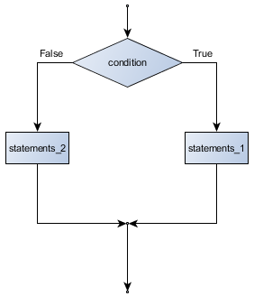
The syntax for an if statement looks like this:
if BOOLEAN EXPRESSION:
    STATEMENTS_1        # Executed if condition evaluates to True
else:
    STATEMENTS_2        # Executed if condition evaluates to False
As with the function definition from the last chapter and other compound statements like for, the if statement consists of a header line and a body. The header line begins with the keyword if followed by a Boolean expression and ends with a colon (:).
The indented statements that follow are called a block. The first unindented statement marks the end of the block.
Each of the statements inside the first block of statements are executed in order if the Boolean expression evaluates to True. The entire first block of statements is skipped if the Boolean expression evaluates to False, and instead all the statements indented under the else clause are executed.
There is no limit on the number of statements that can appear under the two clauses of an if statement, but there has to be at least one statement in each block. Occasionally, it is useful to have a section with no statements (usually as a place keeper, or scaffolding, for code we haven't written yet). In that case, we can use the pass statement, which does nothing except act as a placeholder.
if True:          # This is always True,
    pass          #   so this is always executed, but it does nothing
else:
    pass
Omitting the else clause
Flowchart of an if statement with no else clause
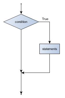
Another form of the if statement is one in which the else clause is omitted entirely. In this case, when the condition evaluates to True, the statements are executed, otherwise the flow of execution continues to the statement after the if.
if x < 0:
    print("The negative number ",  x, " is not valid here.")
    x = 42
    print("I've decided to use the number 42 instead.")

print("The square root of ", x, "is", math.sqrt(x))
In this case, the print function that outputs the square root is the one after the if --- not because we left a blank line, but because of the way the code is indented. Note too that the function call math.sqrt(x) will give an error unless we have an import math statement, usually placed near the top of our script.
Python terminology
Python documentation sometimes uses the term suite of statements to mean what we have called a block here. They mean the same thing, and since most other languages and computer scientists use the word block, we'll stick with that.
Notice too that else is not a statement. The if statement has two clauses, one of which is the (optional) else clause.
The while statement
The if statement allows to make a choice between two blocks of code. However, in a program that only contains assignment and if statements, every statement is still executed at most one. It is very common that we want the computer to repeat statements multiple times. The most basic statement that allows to do so, is the while statement.
However, before introducing the while statement, it is good remind ourselves of some important aspects of assignments.
Assignment vs Boolean Expressions
As we have mentioned previously, it is legal to make more than one assignment to the same variable. A new assignment makes an existing variable refer to a new value (and stop referring to the old value).
airtime_remaining = 15
print(airtime_remaining)
airtime_remaining = 7
print(airtime_remaining)
The output of this program is:
15
7
because the first time airtime_remaining is printed, its value is 15, and the second time, its value is 7.
It is especially important to distinguish between an assignment statement and a Boolean expression that tests for equality. Because Python uses the equal token (=) for assignment, it is tempting to interpret a statement like a = b as a Boolean test. Unlike mathematics, it is not! Remember that the Python token for the equality operator is ==.
Note too that an equality test is symmetric, but assignment is not. For example, if a == 7 then 7 == a. But in Python, the statement a = 7 is legal and 7 = a is not.
In Python, an assignment statement can make two variables equal, but because further assignments can change either of them, they don't have to stay that way:
a = 5
b = a    # After executing this line, a and b are now equal
a = 3    # After executing this line, a and b are no longer equal
The third line changes the value of a but does not change the value of b, so they are no longer equal. (In some programming languages, a different symbol is used for assignment, such as <- or :=, to avoid confusion.) Some people also think that variable was an unfortunate word to choose, and instead we should have called them assignables. Python chooses to follow common terminology and token usage, also found in languages like C, C++, Java, and C#, so we use the tokens = for assignment, == for equality, and we talk of variables.
Updating variables
When an assignment statement is executed, the right-hand side expression (i.e. the expression that comes after the assignment token) is evaluated first. This produces a value. Then the assignment is made, so that the variable on the left-hand side now refers to the new value.
One of the most common forms of assignment is an update, where the new value of the variable depends on its old value.
n = 5
n = 3 * n + 1
Line 2 means get the current value of n, multiply it by three and add one, and assign the answer to n, thus making n refer to the value. So after executing the two lines above, n will point/refer to the integer 16.
If you try to get the value of a variable that has never been assigned to, you'll get an error:
>>> w = x + 1
Traceback (most recent call last):
  File "<interactive input>", line 1, in
NameError: name 'x' is not defined
Before you can update a variable, you have to initialize it to some starting value, usually with a simple assignment:
runs_scored = 0
...
runs_scored = runs_scored + 1
Line 3 --- updating a variable by adding 1 to it --- is very common. It is called an increment of the variable; subtracting 1 is called a decrement. Sometimes programmers also talk about bumping a variable, which means the same as incrementing it by 1.
Structure of the while
Now that we have pointed out some important aspects of assignments, we are ready to introduce the while statement, which allows to repeat lines of code.
Here is a fragment of code that demonstrates the use of the while statement:
n = 4
""" Determine the sum of 1+2+3 ... n """
ss = 0
v = 1
while v <= n:
    ss = ss + v
    v = v + 1
print(v)
When executing this code, the value 10 (1+2+3+4) will be printed on the screen.
You can almost read the while statement as if it were English. It means, while v is less than or equal to n, continue executing the body of the loop. Within the body, each time, increment v. When v passes n, return your accumulated sum.
More formally, here is precise flow of execution for a while statement:
- Evaluate the condition at line 5, yielding a value which is either False or True.
- If the value is False, exit the while statement and continue execution at the next statement (line 8 in this case).
- If the value is True, execute each of the statements in the body (lines 6 and 7) and then go back to the while statement at line 5.
The body consists of all of the statements indented below the while keyword.
Notice that if the loop condition is False the first time we get loop, the statements in the body of the loop are never executed.
The body of the loop should change the value of one or more variables so that eventually the condition becomes false and the loop terminates. Otherwise the loop will repeat forever, which is called an infinite loop. An endless source of amusement for computer scientists is the observation that the directions on shampoo, "lather, rinse, repeat", are an infinite loop.
In the case here, we can prove that the loop terminates because we know that the value of n is finite, and we can see that the value of v increments each time through the loop, so eventually it will have to exceed n. In other cases, it is not so easy, even impossible in some cases, to tell if the loop will ever terminate.
In general, a common construct in many programs is the following:
i = 1
while i <= n:
    STATEMENTS
    i  = i + 1
In this case, we will execute the indicated STATEMENTS n times. However, note that it is possible to use any Boolean expression as a condition; the following is hence also a valid program:
while x >= 0:
    STATEMENTS
    x = x // 2
In this code, we will continue to divide a number x by 2, as long as the outcome of the division is not 2. The power of the while statement is hence that we are very free in how we specify how many times a block of statement is repeated!
Glossary
- block
- A group of consecutive statements with the same indentation.
- body
- The block of statements in a compound statement that follows the header.
- Boolean algebra
- Some rules for rearranging and reasoning about Boolean expressions.
- Boolean expression
- An expression that is either true or false.
- Boolean value
- There are exactly two Boolean values: True and False. Boolean values result when a Boolean expression is evaluated by the Python interepreter. They have type bool.
- branch
- One of the possible paths of the flow of execution determined by conditional execution.
- comparison operator
- One of the six operators that compares two values: ==, !=, >, <, >=, and <=.
- condition
- The Boolean expression in a conditional statement that determines which branch is executed.
- conditional statement
- A statement that controls the flow of execution depending on some condition. In Python the keywords if, elif, and else are used for conditional statements.
- counter
- A variable used to count something, usually initialized to zero and incremented in the body of a loop.
- increment
- Both as a noun and as a verb, increment means to increase by 1.
- infinite loop
- A loop in which the terminating condition is never satisfied.
- indefinite iteration
- A loop where we just need to keep going until some condition is met. A while statement is used for this case.
- iteration
- Repeated execution of a set of programming statements.
- loop
- The construct that allows allows us to repeatedly execute a statement or a group of statements until a terminating condition is satisfied.
- loop variable
- A variable used as part of the terminating condition of a loop.
- logical operator
- One of the operators that combines Boolean expressions: and, or, and not.
- nesting
- One program structure within another, such as a conditional statement inside a branch of another conditional statement.
- prompt
- A visual cue that tells the user that the system is ready to accept input data.
- truth table
- A concise table of Boolean values that can describe the semantics of an operator.
- type conversion
- An explicit function call that takes a value of one type and computes a corresponding value of another type.
References
| [ThinkCS] | How To Think Like a Computer Scientist --- Learning with Python 3 |
Composing expressions and statements
Source: this section is heavily based on Chapter 2 and Chapter 5 of [ThinkCS].
In the previous chapter, we saw a number of types, expressions and statements. More complex programs are created by combining these. In this chapter, we will some of the basics of how to combine types, expressions and statements in more complex manners.
Type converter functions
As indicated earlier, the information that a variable refers to has both a type and a value. Sometimes it is useful to change the value from one type to another. Here we'll look at three more Python functions, int, float and str, which will (attempt to) convert their arguments into types int, float and str respectively. We call these type converter functions.
The int function can take a floating point number or a string, and turn it into an int. For floating point numbers, it discards the decimal portion of the number --- a process we call truncation towards zero on the number line. Let us see this in action:
>>> int(3.14)
3
>>> int(3.9999)             # This doesn't round to the closest int!
3
>>> int(3.0)
3
>>> int(-3.999)             # Note that the result is closer to zero
-3
>>> int(minutes / 60)
10
>>> int("2345")             # Parse a string to produce an int
2345
>>> int(17)                 # It even works if arg is already an int
17
>>> int("23 bottles")
This last case doesn't look like a number --- what do we expect?
Traceback (most recent call last):
File "<interactive input>", line 1, in <module>
ValueError: invalid literal for int() with base 10: '23 bottles'
The type converter float can turn an integer, a float, or a syntactically legal string into a float:
>>> float(17)
17.0
>>> float("123.45")
123.45
The type converter str turns its argument into a string:
>>> str(17)
'17'
>>> str(123.45)
'123.45'
Operations on strings
In general, you cannot perform mathematical operations on strings, even if the strings look like numbers. The following are illegal (assuming that message has type string):
>>> message - 1        # Error
>>> "Hello" / 123      # Error
>>> message * "Hello"  # Error
>>> "15" + 2           # Error
Interestingly, the + operator does work with strings, but for strings, the + operator represents concatenation, not addition. Concatenation means joining the two operands by linking them end-to-end. For example:
fruit = "banana"
baked_good = " nut bread"
print(fruit + baked_good)
The output of this program is banana nut bread. The space before the word nut is part of the string, and is necessary to produce the space between the concatenated strings.
The * operator also works on strings; it performs repetition. For example, 'Fun'*3 is 'FunFunFun'. One of the operands has to be a string; the other has to be an integer.
On one hand, this interpretation of + and * makes sense by analogy with addition and multiplication. Just as 4*3 is equivalent to 4+4+4, we expect "Fun"*3 to be the same as "Fun"+"Fun"+"Fun", and it is. On the other hand, there is a significant way in which string concatenation and repetition are different from integer addition and multiplication. Can you think of a property that addition and multiplication have that string concatenation and repetition do not?
Input
There is a built-in function in Python for getting input from the user:
n = input("Please enter your name: ")
A sample run of this script in Thonny would look like this:
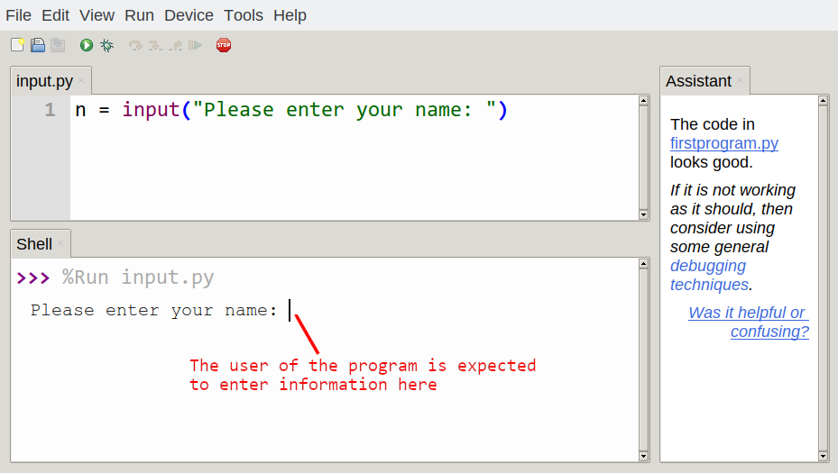
The user of the program can enter the name and press enter, and when this happens the text that has been entered is returned from the input function, and in this case assigned to the variable n.
Even if you asked the user to enter their age, you would get back a string like "17". It would be your job, as the programmer, to convert that string into a int or a float, using the int or float converter functions we saw earlier.
Composition
One of the most useful features of programming languages is their ability to take small building blocks and compose them into larger chunks.
For example, we know how to get the user to enter some input, we know how to convert the string we get into a float, we know how to write a complex expression, and we know how to print values. Let's put these together in a small four-step program that asks the user to input a value for the radius of a circle, and then computes the area of the circle from the formula.

Firstly, we'll do the four steps one at a time:
response = input("What is your radius? ")
r = float(response)
area = 3.14159 * r**2
print("The area is ", area)
Now let's compose the first two lines into a single line of code, and compose the second two lines into another line of code.
r = float( input("What is your radius? ") )
print("The area is ", 3.14159 * r**2)
If we really wanted to be tricky, we could write it all in one statement:
print("The area is ", 3.14159*float(input("What is your radius?"))**2)
Such compact code may not be most understandable for humans, but it does illustrate how we can compose bigger chunks from our building blocks.
If you're ever in doubt about whether to compose code or fragment it into smaller steps, try to make it as simple as you can for the human to follow. My choice would be the first case above, with four separate steps.
The modulus operator
The modulus operator works on integers (and integer expressions) and gives the remainder when the first number is divided by the second. In Python, the modulus operator is a percent sign (%). The syntax is the same as for other operators. It has the same precedence as the multiplication operator.
>>> q = 7 // 3     # This is integer division operator
>>> print(q)
2
>>> r  = 7 % 3
>>> print(r)
1
So 7 divided by 3 is 2 with a remainder of 1.
The modulus operator turns out to be surprisingly useful in larger programs. For example, you can check whether one number is divisible by another---if x % y is zero, then x is divisible by y.
Also, you can extract the right-most digit or digits from a number. For example, x % 10 yields the right-most digit of x (in base 10). Similarly x % 100 yields the last two digits.
It is also extremely useful for doing conversions, say from seconds, to hours, minutes and seconds. So let's write a program to ask the user to enter some seconds, and we'll convert them into hours, minutes, and remaining seconds.
total_secs = int(input("How many seconds, in total?"))
hours = total_secs // 3600
secs_still_remaining = total_secs % 3600
minutes =  secs_still_remaining // 60
secs_finally_remaining = secs_still_remaining  % 60

print("Hrs=", hours, "  mins=", minutes,
                         "secs=", secs_finally_remaining)
Chained conditionals
We have now seen how to combine types and expressions in more complex statements. Similarly, we can also combine if statements in more complex manners. The basic if statement had two branches. Sometimes there are more than two possibilities and we need more than two branches. One way to express a computation like that is a chained conditional:
if x < y:
    STATEMENTS_A
elif x > y:
    STATEMENTS_B
else:
    STATEMENTS_C
Flowchart of this chained conditional
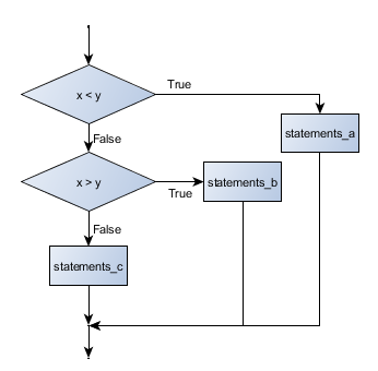
elif is an abbreviation of else if. Again, exactly one branch will be executed. There is no limit of the number of elif statements but only a single (and optional) final else statement is allowed and it must be the last branch in the statement:
if choice == "a":
    function_one()
elif choice == "b":
    function_two()
elif choice == "c":
    function_three()
else:
    print("Invalid choice.")
Each condition is checked in order. If the first is false, the next is checked, and so on. If one of them is true, the corresponding branch executes, and the statement ends. Even if more than one condition is true, only the first true branch executes.
Nested conditionals
One conditional can also be nested within another. (It is the same theme of composability, again!) We could have written the previous example as follows:
Flowchart of this nested conditional
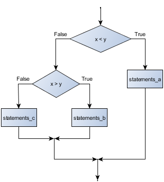
if x < y:
    STATEMENTS_A
else:
    if x > y:
        STATEMENTS_B
    else:
        STATEMENTS_C
The outer conditional contains two branches. The second branch contains another if statement, which has two branches of its own. Those two branches could contain conditional statements as well.
Although the indentation of the statements makes the structure apparent, nested conditionals very quickly become difficult to read. In general, it is a good idea to avoid them when we can.
Logical operators often provide a way to simplify nested conditional statements. For example, we can rewrite the following code using a single conditional:
if 0 < x:            # Assume x is an int here
    if x < 10:
        print("x is a positive single digit.")
The print function is called only if we make it past both the conditionals, so instead of the above which uses two if statements each with a simple condition, we could make a more complex condition using the and operator. Now we only need a single if statement:
if 0 < x and x < 10:
    print("x is a positive single digit.")
Nesting loops and conditionals
Now we have seen that if``s can be nested in each other, it should not come as a surprise that also ``while and if can be nested in each other. Consider the following program:
x = int(input("Provide a number: "))
while x != 0:
    if x < 0:
        print ( -x )
    else:
        print ( x )
    x = int(input("Provide another number: "))
In this code, we continue to ask the user for a number, as long as the user does not enter the number 0. For each such number, we check whether it is positive or negative, and adapt our printing process to the situation. It is perfectly possible to nest the if condition within the while loop.
Also the reverse type of nesting is possible, where we put a while loop within an if block.
Logical opposites
We have already seen how to combine Boolean expressions using and, or and not. Combinations of such expressions can quickly become complex. It is important to then reflect on whether it is possible to simplify such expressions.
Each of the six relational operators has a logical opposite: for example, suppose we can get a driving licence when our age is greater or equal to 17, we can not get the driving licence when we are less than 17.
Notice that the opposite of >= is <.
operator logical opposite == != != == < >= <= > > <= >= <
Understanding these logical opposites allows us to sometimes get rid of not operators. not operators are often quite difficult to read in computer code, and our intentions will usually be clearer if we can eliminate them.
For example, if we wrote this Python:
if not (age >= 17):
    print("Hey, you're too young to get a driving licence!")
it would probably be clearer to use the simplification laws, and to write instead:
if age < 17:
    print("Hey, you're too young to get a driving licence!")
Two powerful simplification laws (called de Morgan's laws) that are often helpful when dealing with complicated Boolean expressions are:
not (x and y)  ==  (not x) or (not y)
not (x or y)   ==  (not x) and (not y)
For example, suppose we can slay the dragon only if our magic lightsabre sword is charged to 90% or higher, and we have 100 or more energy units in our protective shield. We find this fragment of Python code in the game:
if not ((sword_charge >= 0.90) and (shield_energy >= 100)):
    print("Your attack has no effect, the dragon fries you to a crisp!")
else:
    print("The dragon crumples in a heap. You rescue the gorgeous princess!")
de Morgan's laws together with the logical opposites would let us rework the condition in a (perhaps) easier to understand way like this:
if (sword_charge < 0.90) or (shield_energy < 100):
    print("Your attack has no effect, the dragon fries you to a crisp!")
else:
    print("The dragon crumples in a heap. You rescue the gorgeous princess!")
We could also get rid of the not by swapping around the then and else parts of the conditional. So here is a third version, also equivalent:
if (sword_charge >= 0.90) and (shield_energy >= 100):
    print("The dragon crumples in a heap. You rescue the gorgeous princess!")
else:
    print("Your attack has no effect, the dragon fries you to a crisp!")
This version is probably the best of the three, because it very closely matches the initial English statement. Clarity of our code (for other humans), and making it easy to see that the code does what was expected should always be a high priority.
As our programming skills develop we'll find we have more than one way to solve any problem. So good programs are designed. We make choices that favour clarity, simplicity, and elegance. The job title software architect says a lot about what we do --- we are architects who engineer our products to balance beauty, functionality, simplicity and clarity in our creations.
Tip
Once our program works, we should play around a bit trying to polish it up. Write good comments. Think about whether the code would be clearer with different variable names. Could we have done it more elegantly? Should we rather use a function? Can we simplify the conditionals?
We think of our code as our creation, our work of art! We make it great.
Type conversion
We've had a first look at this earlier in this chapter. Seeing it again won't hurt!
Many Python types come with a built-in function that attempts to convert values of another type into its own type. The int function, for example, takes any value and converts it to an integer, if possible, or complains otherwise:
>>> int("32")
32
>>> int("Hello")
ValueError: invalid literal for int() with base 10: 'Hello'
int can also convert floating-point values to integers, but remember that it truncates the fractional part:
>>> int(-2.3)
-2
>>> int(3.99999)
3
>>> int("42")
42
>>> int(1.0)
1
The float function converts integers and strings to floating-point numbers:
>>> float(32)
32.0
>>> float("3.14159")
3.14159
>>> float(1)
1.0
It may seem odd that Python distinguishes the integer value 1 from the floating-point value 1.0. They may represent the same number, but they belong to different types. The reason is that they are represented differently inside the computer.
The str function converts any argument given to it to type string:
>>> str(32)
'32'
>>> str(3.14149)
'3.14149'
>>> str(True)
'True'
>>> str(true)
Traceback (most recent call last):
  File "<interactive input>", line 1, in <module>
NameError: name 'true' is not defined
str will work with any value and convert it into a string. As mentioned earlier, True is Boolean value; true is just an ordinary variable name, and is not defined here, so we get an error.
Glossary
- chained conditional
- A conditional branch with more than two possible flows of execution. In Python chained conditionals are written with if ... elif ... else statements.
- composition
- The ability to combine simple expressions and statements into compound statements and expressions in order to represent complex computations concisely.
- concatenate
- To join two strings end-to-end.
- modulus operator
- An operator, denoted with a percent sign ( %), that works on integers and yields the remainder when one number is divided by another.
References
| [ThinkCS] | How To Think Like a Computer Scientist --- Learning with Python 3 |
Iteration
Source: this section is heavily based on Chapter 7 of [ThinkCS].
Until now we have seen that the while statement can be used for repeatedly executing lines of code. Repeated execution of a set of statements is called iteration. Because iteration is so common, we are going to dive deeper in this topic in this chapter. Among others, we are going to introduce the for statement --- another way to have your program do iteration, useful in slightly different circumstances.
The while loop
Until now, we have seen the while statement for repeating code:
runs_scored = 0
while runs_scored < 5:
    print(runs_scored)
    runs_scored = runs_scored + 1
In this code, we first initialize the variable runs_scored, and then repeatedly increment this variable, until a stop condition is reached. We print the values 0, 1, 2, 3 and 4; then we stop the repetition when runs_scored reaches the value 5. We exploit here the fact that the assignment statement in the loop modifies the value of the variable runs_scored in the memory of the computer.
Note that overall, we repeat the 3rd line in this program 5 times: 1 time when runs_scored==0, one time when runs_scored==1, ..., and 1 time when runs_scored==4 -- 5 in total.
The while statement can always be used to repeat statements. However, it is not always the shortest approach. Python offers an alternative solution: the for loop.
The for loop
In general, we often wish to repeat statements by giving values to one variable. In our earlier example, we repeat the line print(runs_scored) for the values runs_scored==0, runs_scored==1, etc.
The for notation of Python allows us to write this more shortly as follows:
for runs_scored in [0,1,2,3,4]:
    print(runs_scored)
In this code, [0,1,2,3,4] is a list that specifies the values that are going to be assigned to the variable runs_scored; the block of code in the for loop is executed for each value in this list.
While in this example our lists consists of numbers, this need not be the case. We can also iterate over other types. For instance:
for f in ["Joe", "Zoe", "Brad", "Angelina", "Zuki", "Thandi", "Paris"]:
    invitation = "Hi " + f + ".  Please come to my party on Saturday!"
    print(invitation)
Running through all the items in a list is called traversing the list, or traversal.
When we run this, the output looks like this:
Hi Joe.  Please come to my party on Saturday!
Hi Zoe.  Please come to my party on Saturday!
Hi Brad.  Please come to my party on Saturday!
Hi Angelina.  Please come to my party on Saturday!
Hi Zuki.  Please come to my party on Saturday!
Hi Thandi.  Please come to my party on Saturday!
Hi Paris.  Please come to my party on Saturday!
- The variable f in the for statement at line 1 is called the loop variable. We could have chosen any other variable name instead.
- Lines 2 and 3 are the loop body. The loop body is always indented. The indentation determines exactly what statements are "in the body of the loop".
- On each iteration or pass of the loop, we consider one of the elements in the list, and execute the body of the list for that value.
- At the end of each execution of the body of the loop, Python returns to the for statement, to assign the next value to f.
As the program executes, the interpreter always keeps track of which statement is about to be executed. We call this the control flow, of the flow of execution of the program. When humans execute programs, they often use their finger to point to each statement in turn. So we could think of control flow as "Python's moving finger".
Flowchart of a for loop
Control flow is often easy to visualize and understand if we draw a flowchart. This shows the exact steps and logic of how the for statement executes.
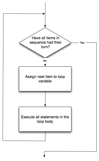
Let us write code now to sum up all the elements in a list of numbers [1.25, 2.5, 1.75]. Do this by hand first, and try to isolate exactly what steps you take. You'll find you need to keep some "running total" of the sum so far, either on a piece of paper, in your head, or in your calculator. Remembering things from one step to the next is precisely why we have variables in a program: so we'll need some variable to remember the "running total". It should be initialized with a value of zero, and then we need to traverse the items in the list. For each item, we'll want to update the running total by adding the next number to it.
""" Sum all the numbers in a list, and print the total. """
running_total = 0
for x in [1.25, 2.5, 1.75]:
    running_total = running_total + x
print(running_total)
The range(n) notation
In the code above, we wrote
for runs_scored in [0,1,2,3,4]:
    print(runs_scored)
It is cumbersome to have to write all the numbers explicitly. Fortunately, Python has a shorthand notation for this, which is the following:
for runs_scored in range(5):
    print(runs_scored)
This code will produce exactly the same output as the previous code. Simple, isn't it?
Actually, not really; most beginning programmers have a very hard time using this notation correctly.
The issue is that we write range(5) with the value 5 to create a list that starts at 0 and ends at 4. There is a good reason for this: the list specified by range(5) contains 5 elements. These 5 elements are 0, 1, 2, 3 and 4.
Consequently, the following code:
for runs_scored in range(5):
    print(runs_scored + 1)
prints the values 1, 2, 3, 4, and 5.
If you are confused by this, you are not alone; you are almost certain to make mistakes with this. However, it is extremely important to understand this correctly for your programs to work correctly.
The Collatz 3n + 1 sequence
As we have now seen, we can iterate using both a for and a while statement. How to make the choice between the two?
Let's look at a sequence that has fascinated and foxed mathematicians for many years. They still cannot answer even quite simple questions about this.
The "computational rule" for creating the sequence is to start from some given n, and to generate the next term of the sequence from n, either by halving n, (whenever n is even), or else by multiplying it by three and adding 1. The sequence terminates when n reaches 1.
This Python function captures that algorithm, where we calculate the sequence for n = 19:
n = 19
""" Print the 3n+1 sequence from n,
    terminating when it reaches 1.
"""
while n != 1:
    print(n, end=", ")
    if n % 2 == 0:        # n is even
        n = n // 2
    else:                 # n is odd
        n = n * 3 + 1
print(n, end=".\n")
Notice first that the print function on line 6 has an extra argument end=", ". This tells the print function to follow the printed string with whatever the programmer chooses (in this case, a comma followed by a space), instead of ending the line. So each time something is printed in the loop, it is printed on the same output line, with the numbers separated by commas. The call to print(n, end=".\n") at line 11 after the loop terminates will then print the final value of n followed by a period and a newline character. (You'll cover the \n (newline character) later).
The condition for continuing with this loop is n != 1, so the loop will continue running until it reaches its termination condition, (i.e. n == 1).
Each time through the loop, the program outputs the value of n and then checks whether it is even or odd. If it is even, the value of n is divided by 2 using integer division. If it is odd, the value is replaced by n * 3 + 1. Here is the output of this program:
19, 58, 29, 88, 44, 22, 11, 34, 17, 52, 26, 13,
                    40, 20, 10, 5, 16, 8, 4, 2, 1.
Since n sometimes increases and sometimes decreases, there is no obvious proof that n will ever reach 1, or that the program terminates. For some particular values of n, we can prove termination. For example, if the starting value is a power of two, then the value of n will be even each time through the loop until it reaches 1. The previous example ends with such a sequence, starting with 16.
See if you can find a small starting number that needs more than a hundred steps before it terminates.
Particular values aside, the interesting question was first posed by a German mathematician called Lothar Collatz: the Collatz conjecture (also known as the 3n + 1 conjecture), is that this sequence terminates for all positive values of n. So far, no one has been able to prove it or disprove it! (A conjecture is a statement that might be true, but nobody knows for sure.)
Think carefully about what would be needed for a proof or disproof of the conjecture "All positive integers will eventually converge to 1 using the Collatz rules". With fast computers we have been able to test every integer up to very large values, and so far, they have all eventually ended up at 1. But who knows? Perhaps there is some as-yet untested number which does not reduce to 1.
You'll notice that if you don't stop when you reach 1, the sequence gets into its own cyclic loop: 1, 4, 2, 1, 4, 2, 1, 4 ... So one possibility is that there might be other cycles that we just haven't found yet.
Wikipedia has an informative article about the Collatz conjecture. The sequence also goes under other names (Hailstone sequence, Wonderous numbers, etc.), and you'll find out just how many integers have already been tested by computer, and found to converge!
Choosing between for and while
Use a for loop if you know, before you start looping, the maximum number of times that you'll need to execute the body. For example, if you're traversing a list of elements, you know that the maximum number of loop iterations you can possibly need is "all the elements in the list". Or if you need to print 12 numbers, we know right away how many times the loop will need to run.
So any problem like "iterate this weather model for 1000 cycles", or "search this list of words", "find all prime numbers up to 10000" suggest that a for loop is best.
By contrast, if you are required to repeat some computation until some condition is met, and you cannot calculate in advance when (of if) this will happen, as we did in this 3n + 1 problem, you'll need a while loop.
We call the first case definite iteration --- we know ahead of time some definite bounds for what is needed. The latter case is called indefinite iteration --- we're not sure how many iterations we'll need --- we cannot even establish an upper bound!
Tracing a program
To write effective computer programs, and to build a good conceptual model of program execution, a programmer needs to develop the ability to trace the execution of a computer program. Tracing involves becoming the computer and following the flow of execution through a sample program run, recording the state of all variables and any output the program generates after each instruction is executed.
To understand this process, let's trace the program from the previous section, with starting value n=3 instead of n=19. At the start of the trace, we have a variable, n (the parameter), with an initial value of 3. Since 3 is not equal to 1, the while loop body is executed. 3 is printed and 3 % 2 == 0 is evaluated. Since it evaluates to False, the else branch is executed and 3 * 3 + 1 is evaluated and assigned to n.
To keep track of all this as you hand trace a program, make a column heading on a piece of paper for each variable created as the program runs and another one for output. Our trace so far would look something like this:
n               output printed so far
--              ---------------------
3               3,
10
Since 10 != 1 evaluates to True, the loop body is again executed, and 10 is printed. 10 % 2 == 0 is true, so the if branch is executed and n becomes 5. By the end of the trace we have:
n               output printed so far
--              ---------------------
3               3,
10              3, 10,
5               3, 10, 5,
16              3, 10, 5, 16,
8               3, 10, 5, 16, 8,
4               3, 10, 5, 16, 8, 4,
2               3, 10, 5, 16, 8, 4, 2,
1               3, 10, 5, 16, 8, 4, 2, 1.
Tracing can be a bit tedious and error prone (that's why we get computers to do this stuff in the first place!), but it is an essential skill for a programmer to have. From this trace we can learn a lot about the way our code works. We can observe that as soon as n becomes a power of 2, for example, the program will require log2(n) executions of the loop body to complete. We can also see that the final 1 will not be printed as output within the body of the loop, which is why we put the special print function at the end.
Tracing a program is, of course, related to single-stepping through your code and being able to inspect the variables. Using the computer to single-step for you is less error prone and more convenient. Also, as your programs get more complex, they might execute many millions of steps before they get to the code that you're really interested in, so manual tracing becomes impossible. Being able to set a breakpoint where you need one is far more powerful. So we strongly encourage you to invest time in learning using to use your programming environment (Thonny, in this course) to full effect.
There are also some great visualization tools becoming available to help you trace and understand small fragments of Python code. The one we recommend is at http://www.pythontutor.com/visualize.html .
Counting digits
Let us consider another example where a while loop is necessary instead of a for loop.
The following code counts the number of decimal digits in a positive integer n, specified by the user:
n = int(input("Give a number:" ))
count = 0
while n != 0:
    count = count + 1
    n = n // 10
print(count)
If the user enters 710, the code will print 3. Trace the execution of this function call (perhaps using the single step function in Thonny, or the Python visualizer, or on some paper) to convince yourself that it works.
This code demonstrates an important pattern of computation called a counter. The variable count is initialized to 0 and then incremented each time the loop body is executed. When the loop exits, count contains the result --- the total number of times the loop body was executed, which is the same as the number of digits.
Note that even though we have a counter here, we cannot use a for loop! In a for loop, we need to specify in advance all the elements we are going to iterate over, but in this case we don't know the end value of count before the loop is executed!
If we wanted to only count digits that are either 0 or 5, adding a conditional before incrementing the counter will do the trick:
n = int(input("Give a number: "))
count = 0
while n > 0:
    digit = n % 10
    if digit == 0 or digit == 5:
        count = count + 1
    n = n // 10
print(count)
Confirm that when we enter 1055030250, as result 7 is printed. What happens when the user enters 0?
Abbreviated assignment
Incrementing a variable is so common that Python provides an abbreviated syntax for it:
>>> count = 0
>>> count += 1
>>> count
1
>>> count += 1
>>> count
2
count += 1 is an abreviation for count = count + 1 . We pronounce the operator as "plus-equals". The increment value does not have to be 1:
>>> n = 2
>>> n += 5
>>> n
7
There are similar abbreviations for -=, *=, /=, //= and %=:
>>> n = 2
>>> n *= 5
>>> n
10
>>> n -= 4
>>> n
6
>>> n //= 2
>>> n
3
>>> n %= 2
>>> n
1
These abbreviations are often used in while loops:
n = int(input("Give a number: "))
while n > 0:
    digit = n % 10
    if digit == 0 or digit == 5:
        count += 1
    n //= 10
print(count)
The break statement
Until now, we have seen that a while loop continues until its condition is no longer True, and a for loop considers all values in a list. Sometimes, however, we wish to stop earlier.
The break statement is used to immediately leave the body of its loop. The next statement to be executed is the first one after the body:
for i in [12, 16, 17, 24, 29]:
    if i % 2 == 1:  # If the number is odd
       break        #  ... immediately exit the loop
    print(i)
print("done")
This prints:
12
16
done
The pre-test loop --- standard loop behaviour
for and while loops do their tests at the start, before executing any part of the body. They're called pre-test loops, because the test happens before (pre) the body. break and return are our tools for adapting this standard behaviour.
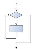
Other flavours of loops
Sometimes we'd like to have the middle-test loop with the exit test in the middle of the body, rather than at the beginning or at the end. Or a post-test loop that puts its exit test as the last thing in the body. Other languages have different syntax and keywords for these different flavours, but Python just uses a combination of while and if condition: break to get the job done.
A typical example is a problem where the user has to input numbers to be summed. To indicate that there are no more inputs, the user enters a special value, often the value -1, or the empty string. This needs a middle-exit loop pattern: input the next number, then test whether to exit, or else process the number:
The middle-test loop flowchart
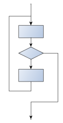
total = 0
while True:
    response = input("Enter the next number. (Leave blank to end)")
    if response == "":
        break
    total += int(response)
print("The total of the numbers you entered is ", total)
Convince yourself that this fits the middle-exit loop flowchart: line 3 does some useful work, lines 4 and 5 can exit the loop, and if they don't line 6 does more useful work before the next iteration starts.
The while bool-expr: uses the Boolean expression to determine whether to iterate again. True is a trivial Boolean expression, so while True: means always do the loop body again. This is a language idiom --- a convention that most programmers will recognize immediately. Since the expression on line 2 will never terminate the loop, (it is a dummy test) the programmer must arrange to break (or return) out of the loop body elsewhere, in some other way (i.e. in lines 4 and 5 in this sample). A clever compiler or interpreter will understand that line 2 is a fake test that must always succeed, so it won't even generate a test, and our flowchart never even put the diamond-shape dummy test box at the top of the loop!
Similarly, by just moving the if condition: break to the end of the loop body we create a pattern for a post-test loop. Post-test loops are used when you want to be sure that the loop body always executes at least once (because the first test only happens at the end of the execution of the first loop body). This is useful, for example, if we want to play an interactive game against the user --- we always want to play at least one game:
while True:
    play_the_game_once()
    response = input("Play again? (yes or no)")
    if response != "yes":
        break
print("Goodbye!")
Hint: Think about where you want the exit test to happen
Once you've recognized that you need a loop to repeat something, think about its terminating condition --- when will I want to stop iterating? Then figure out whether you need to do the test before starting the first (and every other) iteration, or at the end of the first (and every other) iteration, or perhaps in the middle of each iteration. Interactive programs that require input from the user or read from files often need to exit their loops in the middle or at the end of an iteration, when it becomes clear that there is no more data to process, or the user doesn't want to play our game anymore.
An example
The following program implements a simple guessing game:
import random                   # We cover random numbers in the
rng = random.Random()           #  modules chapter, so peek ahead.
number = rng.randrange(1, 1000) # Get random number between [1 and 1000).

guesses = 0
msg = ""

while True:
    guess = int(input(msg + "\nGuess my number between 1 and 1000: "))
    guesses += 1
    if guess > number:
        msg += str(guess) + " is too high.\n"
    elif guess < number:
        msg += str(guess) + " is too low.\n"
    else:
        break

input("\n\nGreat, you got it in {0} guesses!\n\n".format(guesses))
This program makes use of the mathematical law of trichotomy (given real numbers a and b, exactly one of these three must be true: a > b, a < b, or a == b).
At line 18 there is a call to the input function, but we don't do anything with the result, not even assign it to a variable. This is legal in Python. Here it has the effect of popping up the input dialog window and waiting for the user to respond before the program terminates. Programmers often use the trick of doing some extra input at the end of a script, just to keep the window open.
Also notice the use of the msg variable, initially an empty string, on lines 6, 12 and 14. Each time through the loop we extend the message being displayed: this allows us to display the program's feedback right at the same place as we're asking for the next guess.
The continue statement
This is a control flow statement that causes the program to immediately skip the processing of the rest of the body of the loop, for the current iteration. But the loop still carries on running for its remaining iterations:
for i in [12, 16, 17, 24, 29, 30]:
    if i % 2 == 1:      # If the number is odd
       continue         # Don't process it
    print(i)
print("done")
This prints:
12
16
24
30
done
Newton's method for finding square roots
Loops are often used in programs that compute numerical results by starting with an approximate answer and iteratively improving it.
For example, before we had calculators or computers, people needed to calculate square roots manually. Newton used a particularly good method (there is some evidence that this method was known many years before). Suppose that you want to know the square root of n. If you start with almost any approximation, you can compute a better approximation (closer to the actual answer) with the following formula:
better = (approx + n/approx)/2
Repeat this calculation a few times using your calculator. Can you see why each iteration brings your estimate a little closer? One of the amazing properties of this particular algorithm is how quickly it converges to an accurate answer --- a great advantage for doing it manually.
By using a loop and repeating this formula until the better approximation gets close enough to the previous one, we can write a function for computing the square root. (In fact, this is how your calculator finds square roots --- it may have a slightly different formula and method, but it is also based on repeatedly improving its guesses.)
This is an example of an indefinite iteration problem: we cannot predict in advance how many times we'll want to improve our guess --- we just want to keep getting closer and closer. Our stopping condition for the loop will be when our old guess and our improved guess are "close enough" to each other.
Ideally, we'd like the old and new guess to be exactly equal to each other when we stop. But exact equality is a tricky notion in computer arithmetic when real numbers are involved. Because real numbers are not represented absolutely accurately (after all, a number like pi or the square root of two has an infinite number of decimal places because it is irrational), we need to formulate the stopping test for the loop by asking "is a close enough to b"? This stopping condition can be coded like this:
if abs(a-b) < 0.001:  # Make this smaller for better accuracy
      break
Notice that we take the absolute value of the difference between a and b!
This problem is also a good example of when a middle-exit loop is appropriate:
n = float(input("Provide a floating point number: "))
approx = n/2.0     # Start with some or other guess at the answer
while True:
    better = (approx + n/approx)/2.0
    if abs(approx - better) < 0.001:
        return better
    approx = better
The output for input 25.0 is:
5.00000000002
See if you can improve the approximations by changing the stopping condition. Also, step through the algorithm (perhaps by hand, using your calculator) to see how many iterations were needed before it achieved this level of accuracy for sqrt(25).
Algorithms
Newton's method is an example of an algorithm: it is a mechanical process for solving a category of problems (in this case, computing square roots).
Some kinds of knowledge are not algorithmic. For example, learning dates from history or your multiplication tables involves memorization of specific solutions.
But the techniques you learned for addition with carrying, subtraction with borrowing, and long division are all algorithms. Or if you are an avid Sudoku puzzle solver, you might have some specific set of steps that you always follow.
One of the characteristics of algorithms is that they do not require any intelligence to carry out. They are mechanical processes in which each step follows from the last according to a simple set of rules. And they're designed to solve a general class or category of problems, not just a single problem.
Understanding that hard problems can be solved by step-by-step algorithmic processes (and having technology to execute these algorithms for us) is one of the major breakthroughs that has had enormous benefits. So while the execution of the algorithm may be boring and may require no intelligence, algorithmic or computational thinking --- i.e. using algorithms and automation as the basis for approaching problems --- is rapidly transforming our society. Some claim that this shift towards algorithmic thinking and processes is going to have even more impact on our society than the invention of the printing press. And the process of designing algorithms is interesting, intellectually challenging, and a central part of what we call programming.
Some of the things that people do naturally, without difficulty or conscious thought, are the hardest to express algorithmically. Understanding natural language is a good example. We all do it, but so far no one has been able to explain how we do it, at least not in the form of a step-by-step mechanical algorithm.
Glossary
- algorithm
- A step-by-step process for solving a category of problems.
- body
- The statements inside a loop.
- breakpoint
- A place in your program code where program execution will pause (or break), allowing you to inspect the state of the program's variables, or single-step through individual statements, executing them one at a time.
- bump
- Programmer slang. Synonym for increment.
- continue statement
- A statement that causes the remainder of the current iteration of a loop to be skipped. The flow of execution goes back to the top of the loop, evaluates the condition, and if this is true the next iteration of the loop will begin.
- cursor
- An invisible marker that keeps track of where the next character will be printed.
- decrement
- Decrease by 1.
- development plan
- A process for developing a program. In this chapter, we demonstrated a style of development based on developing code to do simple, specific things and then encapsulating and generalizing.
- encapsulate
- To divide a large complex program into components (like functions) and isolate the components from each other (by using local variables, for example).
- escape sequence
- An escape character, \, followed by one or more printable characters used to designate a nonprintable character.
- generalize
- To replace something unnecessarily specific (like a constant value) with something appropriately general (like a variable or parameter). Generalization makes code more versatile, more likely to be reused, and sometimes even easier to write.
- initialization (of a variable)
- To initialize a variable is to give it an initial value. Since in Python variables don't exist until they are assigned values, they are initialized when they are created. In other programming languages this is not the case, and variables can be created without being initialized, in which case they have either default or garbage values.
- loop body
- Any number of statements nested inside a loop. The nesting is indicated by the fact that the statements are indented under the for loop statement.
- loop variable
- A variable used as part of a for loop. It is assigned a different value on each iteration of the loop.
- middle-test loop
- A loop that executes some of the body, then tests for the exit condition, and then may execute some more of the body. We don't have a special Python construct for this case, but can use while and break together.
- nested loop
- A loop inside the body of another loop.
- newline
- A special character that causes the cursor to move to the beginning of the next line.
- post-test loop
- A loop that executes the body, then tests for the exit condition. We don't have a special Python construct for this, but can use while and break together.
- pre-test loop
- A loop that tests before deciding whether the execute its body. for and while are both pre-test loops.
- range
- A built-in function in Python for generating sequences of integers. It is especially useful when we need to write a for loop that executes a fixed number of times.
- single-step
- A mode of interpreter execution where you are able to execute your program one step at a time, and inspect the consequences of that step. Useful for debugging and building your internal mental model of what is going on.
- tab
- A special character that causes the cursor to move to the next tab stop on the current line.
- trichotomy
- Given any real numbers a and b, exactly one of the following relations holds: a < b, a > b, or a == b. Thus when you can establish that two of the relations are false, you can assume the remaining one is true.
- trace
- To follow the flow of execution of a program by hand, recording the change of state of the variables and any output produced.
- terminating condition
- A condition that occurs which causes a loop to stop repeating its body. In the for loops we saw in this chapter, the terminating condition has been when there are no more elements to assign to the loop variable.
References
| [ThinkCS] | How To Think Like a Computer Scientist --- Learning with Python 3 |
Hello, little turtles!
Source: this section is heavily based on Chapter 3 of [ThinkCS].
There are many modules in Python that provide very powerful features that we can use in our own programs. Some of these can send email, or fetch web pages. The one we'll look at in this chapter allows us to create turtles and get them to draw shapes and patterns.
The turtles are fun, but the real purpose of the chapter is to teach ourselves a little more Python, and to develop our theme of computational thinking, or thinking like a computer scientist. Most of the Python covered here will be explored in more depth later.
Our first turtle program
Let's write a couple of lines of Python program to create a new turtle and start drawing a rectangle. (We'll call the variable that refers to our first turtle alex, but we can choose another name if we follow the naming rules from the previous chapter).
import turtle             # Allows us to use turtles
wn = turtle.Screen()      # Creates a playground for turtles
alex = turtle.Turtle()    # Create a turtle, assign to alex

alex.forward(50)          # Tell alex to move forward by 50 units
alex.left(90)             # Tell alex to turn by 90 degrees
alex.forward(30)          # Complete the second side of a rectangle

wn.mainloop()             # Wait for user to close window
When we run this program, a new window pops up:
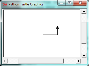
Here are a couple of things we'll need to understand about this program.
The first line tells Python to load a module named turtle. That module brings us two new types that we can use: the Turtle type, and the Screen type. The dot notation turtle.Turtle means "The Turtle type that is defined within the turtle module". (Remember that Python is case sensitive, so the module name, with a lowercase t, is different from the type Turtle.)
We then create and open what it calls a screen (we would prefer to call it a window), which we assign to variable wn. Every window contains a canvas, which is the area inside the window on which we can draw.
In line 3 we create a turtle. The variable alex is made to refer to this turtle.
So these first three lines have set things up, we're ready to get our turtle to draw on our canvas.
In lines 5-7, we instruct the object alex to move, and to turn. We do this by invoking, or activating, alex's methods --- these are the instructions that all turtles know how to respond to.
The last line plays a part too: the wn variable refers to the window shown above. When we invoke its mainloop method, it enters a state where it waits for events (like keypresses, or mouse movement and clicks). The program will terminate when the user closes the window.
An object can have various methods --- things it can do --- and it can also have attributes --- (sometimes called properties). For example, each turtle has a color attribute. The method invocation alex.color("red") will make alex red, and drawing will be red too. (Note the word color is spelled the American way!)
The color of the turtle, the width of its pen, the position of the turtle within the window, which way it is facing, and so on are all part of its current state. Similarly, the window object has a background color, and some text in the title bar, and a size and position on the screen. These are all part of the state of the window object.
Quite a number of methods exist that allow us to modify the turtle and the window objects. We'll just show a couple. In this program we've only commented those lines that are different from the previous example (and we've used a different variable name for this turtle):
import turtle
wn = turtle.Screen()
wn.bgcolor("lightgreen")      # Set the window background color
wn.title("Hello, Tess!")      # Set the window title

tess = turtle.Turtle()
tess.color("blue")            # Tell tess to change her color
tess.pensize(3)               # Tell tess to set her pen width

tess.forward(50)
tess.left(120)
tess.forward(50)

wn.mainloop()
When we run this program, a new window pops up, and will remain on the screen until we close it.
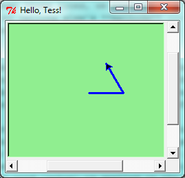
Extend this program ...
- Modify this program so that before it creates the window, it prompts the user to enter the desired background color. It should store the user's responses in a variable, and modify the color of the window according to the user's wishes. (Hint: you can find a list of permitted color names at http://www.tcl.tk/man/tcl8.4/TkCmd/colors.htm. It includes some quite unusual ones, like "peach puff" and "HotPink".)
- Do similar changes to allow the user, at runtime, to set tess' color.
- Do the same for the width of tess' pen. Hint: your dialog with the user will return a string, but tess' pensize method expects its argument to be an int. So you'll need to convert the string to an int before you pass it to pensize.
Instances --- a herd of turtles
Just like we can have many different integers in a program, we can have many turtles. Each of them is called an instance. Each instance has its own attributes and methods --- so alex might draw with a thin black pen and be at some position, while tess might be going in her own direction with a fat pink pen.
import turtle
wn = turtle.Screen()         # Set up the window and its attributes
wn.bgcolor("lightgreen")
wn.title("Tess & Alex")

tess = turtle.Turtle()       # Create tess and set some attributes
tess.color("hotpink")
tess.pensize(5)

alex = turtle.Turtle()       # Create alex

tess.forward(80)             # Make tess draw equilateral triangle
tess.left(120)
tess.forward(80)
tess.left(120)
tess.forward(80)
tess.left(120)               # Complete the triangle

tess.right(180)              # Turn tess around
tess.forward(80)             # Move her away from the origin

alex.forward(50)             # Make alex draw a square
alex.left(90)
alex.forward(50)
alex.left(90)
alex.forward(50)
alex.left(90)
alex.forward(50)
alex.left(90)

wn.mainloop()
Here is what happens when alex completes his rectangle, and tess completes her triangle:
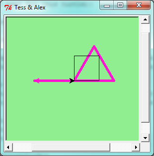
Here are some How to think like a computer scientist observations:
- There are 360 degrees in a full circle. If we add up all the turns that a turtle makes, no matter what steps occurred between the turns, we can easily figure out if they add up to some multiple of 360. This should convince us that alex is facing in exactly the same direction as he was when he was first created. (Geometry conventions have 0 degrees facing East, and that is the case here too!)
- We could have left out the last turn for alex, but that would not have been as satisfying. If we're asked to draw a closed shape like a square or a rectangle, it is a good idea to complete all the turns and to leave the turtle back where it started, facing the same direction as it started in. This makes reasoning about the program and composing chunks of code into bigger programs easier for us humans!
- We did the same with tess: she drew her triangle, and turned through a full 360 degrees. Then we turned her around and moved her aside. Even the blank line 18 is a hint about how the programmer's mental chunking is working: in big terms, tess' movements were chunked as "draw the triangle" (lines 12-17) and then "move away from the origin" (lines 19 and 20).
- One of the key uses for comments is to record our mental chunking, and big ideas. They're not always explicit in the code.
- And, uh-huh, two turtles may not be enough for a herd. But the important idea is that the turtle module gives us a kind of factory that lets us create as many turtles as we need. Each instance has its own state and behaviour.
The loop simplifies our turtle program
To draw a square we'd like to do the same thing four times --- move the turtle, and turn. We previously used 8 lines to have alex draw the four sides of a square. This does exactly the same, but using just three lines:
for i in [0,1,2,3]:
    alex.forward(50)
    alex.left(90)
Some observations:
While "saving some lines of code" might be convenient, it is not the big deal here. What is much more important is that we've found a "repeating pattern" of statements, and reorganized our program to repeat the pattern. Finding the chunks and somehow getting our programs arranged around those chunks is a vital skill in computational thinking.
The values [0,1,2,3] were provided to make the loop body execute 4 times. We could have used any four values, but these are the conventional ones to use. We could have also used range:
for i in range(4):
    # Executes the body with i = 0, then 1, then 2, then 3
for x in range(10):
    # Sets x to each of ... [0, 1, 2, 3, 4, 5, 6, 7, 8, 9]
Our little trick earlier to make sure that alex did the final turn to complete 360 degrees has paid off: if we had not done that, then we would not have been able to use a loop for the fourth side of the square. It would have become a "special case", different from the other sides. When possible, we'd much prefer to make our code fit a general pattern, rather than have to create a special case.
So to repeat something four times, a good Python programmer would do this:
for i in range(4):
    alex.forward(50)
    alex.left(90)
By now you should be able to see how to change our previous program so that tess can also use a for loop to draw her equilateral triangle.
But now, what would happen if we made this change?
for c in ["yellow", "red", "purple", "blue"]:
    alex.color(c)
    alex.forward(50)
    alex.left(90)
A variable can also be assigned a value that is a list. So lists can also be used in more general situations, not only in the for loop. The code above could be rewritten like this:
# Assign a list to a variable
clrs = ["yellow", "red", "purple", "blue"]
for c in clrs:
    alex.color(c)
    alex.forward(50)
    alex.left(90)
A few more turtle methods and tricks
Turtle methods can use negative angles or distances. So tess.forward(-100) will move tess backwards, and tess.left(-30) turns her to the right. Additionally, because there are 360 degrees in a circle, turning 30 to the left will get tess facing in the same direction as turning 330 to the right! (The on-screen animation will differ, though --- you will be able to tell if tess is turning clockwise or counter-clockwise!)
This suggests that we don't need both a left and a right turn method --- we could be minimalists, and just have one method. There is also a backward method. (If you are very nerdy, you might enjoy saying alex.backward(-100) to move alex forward!)
Part of thinking like a scientist is to understand more of the structure and rich relationships in our field. So revising a few basic facts about geometry and number lines, and spotting the relationships between left, right, backward, forward, negative and positive distances or angles values is a good start if we're going to play with turtles.
A turtle's pen can be picked up or put down. This allows us to move a turtle to a different place without drawing a line. The methods are
alex.penup()
alex.forward(100)     # This moves alex, but no line is drawn
alex.pendown()
Every turtle can have its own shape. The ones available "out of the box" are arrow, blank, circle, classic, square, triangle, turtle.
alex.shape("turtle")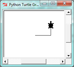
We can speed up or slow down the turtle's animation speed. (Animation controls how quickly the turtle turns and moves forward). Speed settings can be set between 1 (slowest) to 10 (fastest). But if we set the speed to 0, it has a special meaning --- turn off animation and go as fast as possible.
alex.speed(10)
A turtle can "stamp" its footprint onto the canvas, and this will remain after the turtle has moved somewhere else. Stamping works, even when the pen is up.
Let's do an example that shows off some of these new features:
import turtle
wn = turtle.Screen()
wn.bgcolor("lightgreen")
tess = turtle.Turtle()
tess.shape("turtle")
tess.color("blue")

tess.penup()                # This is new
size = 20
for i in range(30):
   tess.stamp()             # Leave an impression on the canvas
   size = size + 3          # Increase the size on every iteration
   tess.forward(size)       # Move tess along
   tess.right(24)           #  ...  and turn her

wn.mainloop()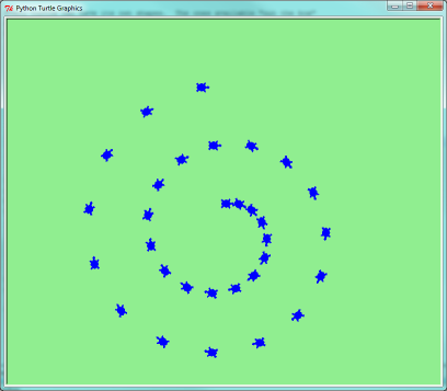
Be careful now! How many times was the body of the loop executed? How many turtle images do we see on the screen? All except one of the shapes we see on the screen here are footprints created by stamp. But the program still only has one turtle instance --- can you figure out which one here is the real tess? (Hint: if you're not sure, write a new line of code after the for loop to change tess' color, or to put her pen down and draw a line, or to change her shape, etc.)
Glossary
- attribute
- Some state or value that belongs to a particular object. For example, tess has a color.
- canvas
- A surface within a window where drawing takes place.
- instance
- An object of a certain type, or class. tess and alex are different instances of the class Turtle.
- method
- A function that is attached to an object. Invoking or activating the method causes the object to respond in some way, e.g. forward is the method when we say tess.forward(100).
- invoke
- An object has methods. We use the verb invoke to mean activate the method. Invoking a method is done by putting parentheses after the method name, with some possible arguments. So tess.forward() is an invocation of the forward method.
- module
- A file containing Python definitions and statements intended for use in other Python programs. The contents of a module are made available to the other program by using the import statement.
- object
- A "thing" to which a variable can refer. This could be a screen window, or one of the turtles we have created.
References
| [ThinkCS] | How To Think Like a Computer Scientist --- Learning with Python 3 |
Functions
Source: this section is heavily based on Chapter 4 of [ThinkCS].
Motivation
In an earlier chapter, we saw the following code:
n = int(input("Give a number: "))
count = 0
while n > 0:
    count = count + 1
    n = n // 10
print(count)
This code allowed the user to type in a number, performed a calculation on this number, and then printed the outcome of this calculation.
In this specific case, we were counting the number of digits in the decimal representation of an integer.
While this code is readable, and has desired functionality, most programmers do not consider this good code.
As a programmer you will often have to write programs that provide additional and more complex functionality than this. For instance, suppose we are implementing a calculator, and this calculator should implement additional functionality such as addition, subtraction, multiplication, division, sinus, cosinus...; such a program would become very long very quickly. We need some approach to structure code if many different functionalities have to be implemented.
The core building block in Python for organising the functionality of your code, is to divide your code into functions. In Python, a function is a named sequence of statements that belong together. Their primary purpose is to help us organize programs into chunks that match how we think about the problem.
For our earlier example, this is one way to write this code in an equivalent manner using a function:
def ndigits ( n ):
    count = 0
    while n > 0:
        count = count + 1
        n = n // 10
    return count

number = int(input("Give a number: "))
print(ndigits(number))
What we have done here, is that we have given a name to our calculation, ndigits. We have specified that the code of this calculation operates on a variable n. At the end of the calculation, we indicate that the outcome of the calculation is what is stored in the variable n.
Subsequently, in the unnamed part of our code we ask the user of our program to type in a number; for this number, we execute the ndigits function, and we print the outcome of the calculation. Note that when we execute this program, it will start by asking the user to give a number; the code within our function ndigits is not (yet) executed: this will only happen after the user has typed in a number, in the last line of the program.
The structure of this code is better. We have separated the user interaction from the calculation; it is now clear which chunk of the code calculates the number of digits.
Now it is easier to extend the program, for instance, consider this program:
def ndigits ( n ):
    count = 0
    while n > 0:
        count = count + 1
        n = n // 10
    return count

def sumdigits ( n ):
    digitsum = 0
    while n > 0:
        digitsum = digitsum + n % 10
        n = n // 10
    return digitsum

number = int(input("Give a number: "))
choice = int(input("Do you want to calculate the number of digits (1) or to sum the digits (2): "))
if choice == 1:
    print(ndigits(number))
if choice == 2:
    print(sumdigits(number))
Here we have added second functionality to our program. Study for yourself what this functionality does!
Moreover, it is easier to reuse code now. For instance, consider the following code:
def ndigits ( n ):
    count = 0
    while n > 0:
        count = count + 1
        n = n // 10
    return count

for i in [344,23,3493]:
    print(ndigits(i))
Our function ndigits has not changed; we only changed how it is used. In this particular case, we print the number of digits for 3 integers.
It is sometimes said that programmers are lazy; this is true. Most programmers want to write the same code only once. Functions allow you to do so and be lazy.
The core insight we had here is that the calculation done in ndigits could be used in a number of different ways; it is useful to put this code together and give it a name, such that we can reuse it.
Let's now consider what a function in general looks like.
Syntax
The general syntax for a function definition is:
def NAME( PARAMETERS ):
    STATEMENTS
We can make up any names we want for the functions we create, except that we can't use a name that is a Python keyword, and the names must follow the rules for legal identifiers.
There can be any number of statements inside the function, but they have to be indented from the def. In the examples in this book, we will use the standard indentation of four spaces. Function definitions are the second of several compound statements we will see, all of which have the same pattern:
- A header line which begins with a keyword and ends with a colon.
- A body consisting of one or more Python statements, each indented the same amount --- the Python style guide recommends 4 spaces --- from the header line.
We've already seen the for loop which follows this pattern.
So looking again at the function definition, the keyword in the header is def, which is followed by the name of the function and some parameters enclosed in parentheses. The parameter list may be empty, or it may contain any number of parameters separated from one another by commas. In either case, the parentheses are required. The parameters specifies what information, if any, we have to provide in order to use the new function.
A Turtle Example
Suppose we're working with turtles, and a common operation we need is to draw squares. "Draw a square" is an abstraction, or a mental chunk, of a number of smaller steps. So let's write a function to capture the pattern of this "building block":
import turtle

def draw_square(t, sz):
    """Make turtle t draw a square of sz."""
    for i in range(4):
        t.forward(sz)
        t.left(90)


wn = turtle.Screen()        # Set up the window and its attributes
wn.bgcolor("lightgreen")
wn.title("Alex meets a function")

alex = turtle.Turtle()      # Create alex
draw_square(alex, 50)       # Call the function to draw the square
wn.mainloop()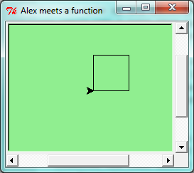
This function is named draw_square. It has two parameters: one to tell the function which turtle to move around, and the other to tell it the size of the square we want drawn. Make sure you know where the body of the function ends --- it depends on the indentation, and the blank lines don't count for this purpose!
Docstrings for documentation
If the first thing after the function header is a string, it is treated as a docstring and gets special treatment in Python and in some programming tools. .. For example, when we type a built-in function name with an unclosed parenthesis in Tonny (Not), a tooltip pops up, telling us what arguments the function takes, and it shows us any other text contained in the docstring.
Docstrings are the key way to document our functions in Python and the documentation part is important. Because whoever calls our function shouldn't have to need to know what is going on in the function or how it works; they just need to know what arguments our function takes, what it does, and what the expected result is. Enough to be able to use the function without having to look underneath. This goes back to the concept of abstraction of which we'll talk more about.
Docstrings are usually formed using triple-quoted strings as they allow us to easily expand the docstring later on should we want to write more than a one-liner.
Just to differentiate from comments, a string at the start of a function (a docstring) is retrievable by Python tools at runtime. By contrast, comments are completely eliminated when the program is parsed.
Defining a new function does not make the function run. To do that we need a function call. We've already seen how to call some built-in functions like print, range and int. Function calls contain the name of the function being executed followed by a list of values, called arguments, which are assigned to the parameters in the function definition. So in the second last line of the program, we call the function, and pass alex as the turtle to be manipulated, and 50 as the size of the square we want. While the function is executing, then, the variable sz refers to the value 50, and the variable t refers to the same turtle instance that the variable alex refers to.
Once we've defined a function, we can call it as often as we like, and its statements will be executed each time we call it. And we could use it to get any of our turtles to draw a square. In the next example, we've changed the draw_square function a little, and we get tess to draw 15 squares, with some variations.
import turtle

def draw_multicolor_square(t, sz):
    """Make turtle t draw a multi-color square of sz."""
    for i in ["red", "purple", "hotpink", "blue"]:
        t.color(i)
        t.forward(sz)
        t.left(90)

wn = turtle.Screen()        # Set up the window and its attributes
wn.bgcolor("lightgreen")

tess = turtle.Turtle()      # Create tess and set some attributes
tess.pensize(3)

size = 20                   # Size of the smallest square
for i in range(15):
    draw_multicolor_square(tess, size)
    size = size + 10        # Increase the size for next time
    tess.forward(10)        # Move tess along a little
    tess.right(18)          #    and give her some turn

wn.mainloop()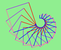
Functions can call other functions
Let's assume now we want a function to draw a rectangle. We need to be able to call the function with different arguments for width and height. And, unlike the case of the square, we cannot repeat the same thing 4 times, because the four sides are not equal.
So we eventually come up with this rather nice code that can draw a rectangle.
def draw_rectangle(t, w, h):
    """Get turtle t to draw a rectangle of width w and height h."""
    for i in range(2):
        t.forward(w)
        t.left(90)
        t.forward(h)
        t.left(90)
The parameter names are deliberately chosen as single letters to ensure they're not misunderstood. In real programs, once we've had more experience, we will insist on better variable names than this. But the point is that the program doesn't "understand" that we're drawing a rectangle, or that the parameters represent the width and the height. Concepts like rectangle, width, and height are the meaning we humans have, not concepts that the program or the computer understands.
Thinking like a scientist involves looking for patterns and relationships. In the code above, we've done that to some extent. We did not just draw four sides. Instead, we spotted that we could draw the rectangle as two halves, and used a loop to repeat that pattern twice.
But now we might spot that a square is a special kind of rectangle. We already have a function that draws a rectangle, so we can use that to draw our square.
def draw_square(tx, sz):        # A new version of draw_square
    draw_rectangle(tx, sz, sz)
There are some points worth noting here:
- Functions can call other functions.
- Rewriting draw_square like this captures the relationship that we've spotted between squares and rectangles.
- A caller of this function might say draw_square(tess, 50). The parameters of this function, tx and sz, are assigned the values of the tess object, and the int 50 respectively.
- In the body of the function they are just like any other variable.
- When the call is made to draw_rectangle, the values in variables tx and sz are fetched first, then the call happens. So as we enter the top of function draw_rectangle, its variable t is assigned the tess object, and w and h in that function are both given the value 50.
So far, it may not be clear why it is worth the trouble to create all of these new functions. Actually, there are a lot of reasons, but this example demonstrates two:
- Creating a new function gives us an opportunity to name a group of statements. Functions can simplify a program by hiding a complex computation behind a single command. The function (including its name) can capture our mental chunking, or abstraction, of the problem.
- Creating a new function can make a program smaller by eliminating repetitive code.
As we might expect, we have to create a function before we can execute it. In other words, the function definition has to be executed before the function is called.
Flow of execution
In order to ensure that a function is defined before its first use, we have to know the order in which statements are executed, which is called the flow of execution. We've already talked about this a little in an earlier chapter.
Execution always begins at the first statement of the program. Statements are executed one at a time, in order from top to bottom.
Function definitions do not alter the flow of execution of the program, but remember that statements inside the function are not executed until the function is called. Although it is not common, we can define one function inside another. In this case, the inner definition isn't executed until the outer function is called.
Function calls are like a detour in the flow of execution. Instead of going to the next statement, the flow jumps to the first line of the called function, executes all the statements there, and then comes back to pick up where it left off.
That sounds simple enough, until we remember that one function can call another. While in the middle of one function, the program might have to execute the statements in another function. But while executing that new function, the program might have to execute yet another function!
Fortunately, Python is adept at keeping track of where it is, so each time a function completes, the program picks up where it left off in the function that called it. When it gets to the end of the program, it terminates.
What's the moral of this sordid tale? When we read a program, don't read from top to bottom. Instead, follow the flow of execution.
Watch the flow of execution in action
In Thonny, we can watch the flow of execution by "stepping" through any program. Thonny will highlight the code that is being executed and will show the values of the variables. One can also enable a view of all the variables in a side pane of the tool.
This is a powerful mechanism for building a deep and thorough understanding of what is happening at each step of the way. Learn to use stepping feature well, and be mentally proactive: as you work through the code, challenge yourself before each step: "What changes will this line make to any variables in the program?" and "Where will flow of execution go next?"
Let us go back and see how this works with the program above that draws 15 multicolor squares. First, we're going to add one line of magic below the import statement --- not strictly necessary, but it will make our lives much simpler, because it prevents stepping into the module containing the turtle code.
import turtle
__import__("turtle").__traceable__ = False
Now we're ready to begin. Put the mouse cursor on the line number of the line where we create the turtle screen, and double click. A red circle will appear; this indicates we wish to stop the execution of the progam at this line. Subsequently, start debugging the program by pressing the "debug" button. This will run the Python program up to, but not including, the line where we have put the red circle. Our program will "break" now, and provide a highlight on the next line to be executed, something like this:
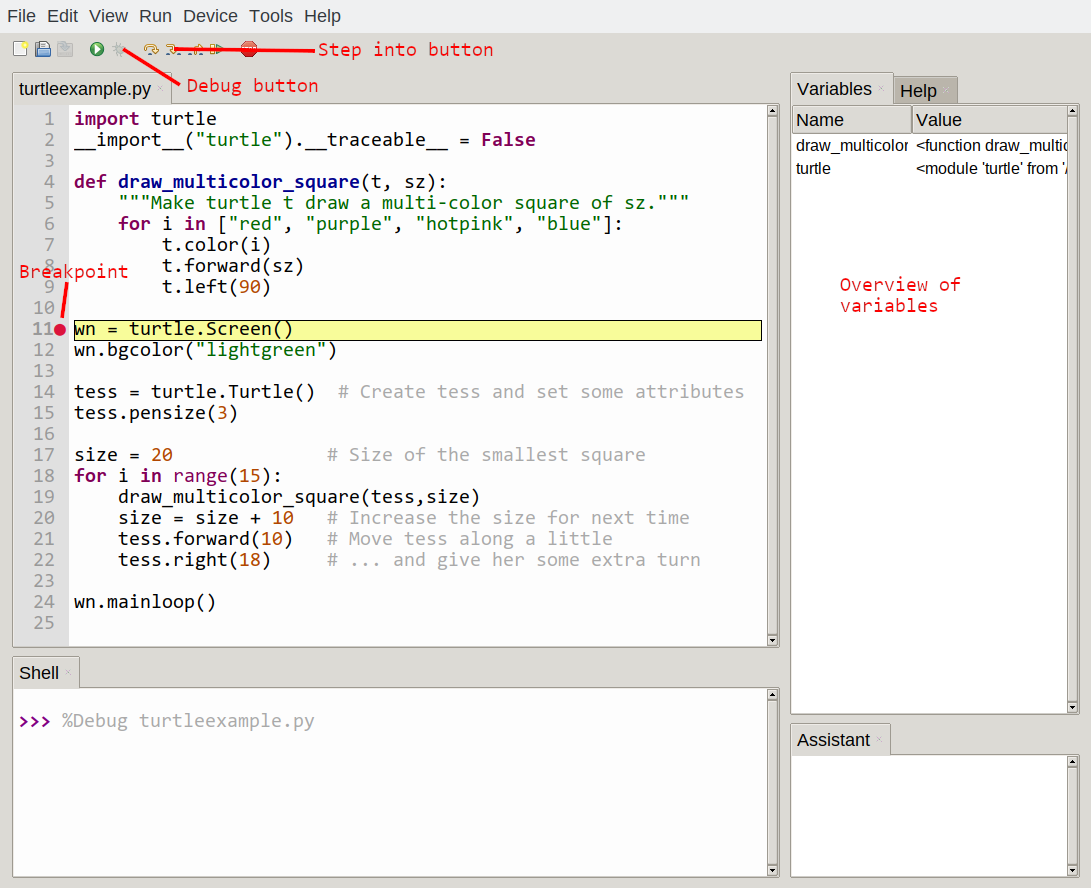
At this point we can press the F7 key (step into) repeatedly to single step through the code. Observe as we execute lines 10, 11, 12, ... how the turtle window gets created, how its canvas color is changed, how the title gets changed, how the turtle is created on the canvas, and then how the flow of execution gets into the loop, and from there into the function, and into the function's loop, and then repeatedly through the body of that loop.
While we do this, we also see the values of the variables, and can confirm that their values match our conceptual model of what is happening.
After a few loops, when we're about to execute line 20 and we're starting to get bored, we can use the key F6 to "step over" the function we are calling. This executes all the statements in the function, but without having to step through each one. We always have the choice to either "go for the detail", or to "take the high-level view" and execute the function as a single chunk.
There are some other options, including one that allow us to resume execution without further stepping.
Functions that require arguments
Most functions require arguments: the arguments provide for generalization. For example, if we want to find the absolute value of a number, we have to indicate what the number is. Python has a built-in function for computing the absolute value:
>>> abs(5)
5
>>> abs(-5)
5
In this example, the arguments to the abs function are 5 and -5.
Some functions take more than one argument. For example the built-in function pow takes two arguments, the base and the exponent. Inside the function, the values that are passed get assigned to variables called parameters.
>>> pow(2, 3)
8
>>> pow(7, 4)
2401
Another built-in function that takes more than one argument is max.
>>> max(7, 11)
11
>>> max(4, 1, 17, 2, 12)
17
>>> max(3 * 11, 5**3, 512 - 9, 1024**0)
503
max can be passed any number of arguments, separated by commas, and will return the largest value passed. The arguments can be either simple values or expressions. In the last example, 503 is returned, since it is larger than 33, 125, and 1.
Functions that return values
All the functions in the previous section return values. Furthermore, functions like range, int, abs all return values that can be used to build more complex expressions.
So an important difference between these functions and one like draw_square is that draw_square was not executed because we wanted it to compute a value --- on the contrary, we wrote draw_square because we wanted it to execute a sequence of steps that caused the turtle to draw.
A function that returns a value is called a fruitful function in this book. The opposite of a fruitful function is void function --- one that is not executed for its resulting value, but is executed because it does something useful. (Languages like Java, C#, C and C++ use the term "void function", other languages like Pascal call it a procedure.) Even though void functions are not executed for their resulting value, Python always wants to return something. So if the programmer doesn't arrange to return a value, Python will automatically return the value None.
How do we write our own fruitful function? In an earlier chapter we saw the standard formula for compound interest, which we'll now write as a fruitful function:
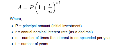 def final_amt(p, r, n, t): """ Apply the compound interest formula to p to produce the final amount. """ a = p * (1 + r/n) ** (n*t) return a # This is new, and makes the function fruitful. # now that we have the function above, let us call it. toInvest = float(input("How much do you want to invest?")) fnl = final_amt(toInvest, 0.08, 12, 5) print("At the end of the period you'll have", fnl)
The return statement is followed by an expression (a in this case). This expression will be evaluated and returned to the caller as the "fruit" of calling this function.
We prompted the user for the principal amount. The type of toInvest is a string, but we need a number before we can work with it. Because it is money, and could have decimal places, we've used the float type converter function to parse the string and return a float.
Notice how we entered the arguments for 8% interest, compounded 12 times per year, for 5 years.
When we run this, we get the output
At the end of the period you'll have 14898.457083
This is a bit messy with all these decimal places, but remember that Python doesn't understand that we're working with money: it just does the calculation to the best of its ability, without rounding. Later we'll see how to format the string that is printed in such a way that it does get nicely rounded to two decimal places before printing.
The line toInvest = float(input("How much do you want to invest?")) also shows yet another example of composition --- we can call a function like float, and its arguments can be the results of other function calls (like input) that we've called along the way.
Note how also in this example we have separated the user interaction from the calculation, which is done in the function, as in the example at the beginning of this chapter.
Notice something else very important here. The name of the variable we pass as an argument --- toInvest --- has nothing to do with the name of the parameter --- p. It is as if p = toInvest is executed when final_amt is called. It doesn't matter what the value was named in the caller, in final_amt its name is p.
These short variable names are getting quite tricky, so perhaps we'd prefer one of these versions instead:
def final_amt_v2(principalAmount, nominalPercentageRate,
                                    numTimesPerYear, years):
    a = principalAmount * (1 + nominalPercentageRate /
                         numTimesPerYear) ** (numTimesPerYear*years)
    return a

def final_amt_v3(amt, rate, compounded, years):
    a = amt * (1 + rate/compounded) ** (componded*years)
    return a
They all do the same thing. Use your judgement to write code that can be best understood by other humans! Short variable names are more economical and sometimes make code easier to read: E = mc2 would not be nearly so memorable if Einstein had used longer variable names! If you do prefer short names, make sure you also have some comments to enlighten the reader about what the variables are used for.
Variables and parameters are local
When we create a local variable inside a function, it only exists inside the function, and we cannot use it outside. For example, consider again this function:
def final_amt(p, r, n, t):
    a = p * (1 + r/n) ** (n*t)
    return a
If we try to use a, outside the function, we'll get an error:
>>> a
NameError: name 'a' is not defined
The variable a is local to final_amt, and is not visible outside the function.
Additionally, a only exists while the function is being executed --- we call this its lifetime. When the execution of the function terminates, the local variables are destroyed.
Parameters are also local, and act like local variables. For example, the lifetimes of p, r, n, t begin when final_amt is called, and the lifetime ends when the function completes its execution.
So it is not possible for a function to set some local variable to a value, complete its execution, and then when it is called again next time, recover the local variable. Each call of the function creates new local variables, and their lifetimes expire when the function returns to the caller.
Turtles Revisited
Now that we have fruitful functions, we can focus our attention on reorganizing our code so that it fits more nicely into our mental chunks. This process of rearrangement is called refactoring the code.
Two things we're always going to want to do when working with turtles is to create the window for the turtle, and to create one or more turtles. We could write some functions to make these tasks easier in future:
def make_window(colr, ttle):
    """
      Set up the window with the given background color and title.
      Returns the new window.
    """
    w = turtle.Screen()
    w.bgcolor(colr)
    w.title(ttle)
    return w


def make_turtle(colr, sz):
    """
      Set up a turtle with the given color and pensize.
      Returns the new turtle.
    """
    t = turtle.Turtle()
    t.color(colr)
    t.pensize(sz)
    return t


wn = make_window("lightgreen", "Tess and Alex dancing")
tess = make_turtle("hotpink", 5)
alex = make_turtle("black", 1)
dave = make_turtle("yellow", 2)
The trick about refactoring code is to anticipate which things we are likely to want to change each time we call the function: these should become the parameters, or changeable parts, of the functions we write.
A Turtle Bar Chart
The turtle has a lot more power than we've seen so far. The full documentation can be found at https://docs.python.org/3/library/turtle.html.
Here are a couple of new tricks for our turtles:
- We can get a turtle to display text on the canvas at the turtle's current position. The method to do that is alex.write("Hello").
- We can fill a shape (circle, semicircle, triangle, etc.) with a color. It is a two-step process. First we call the method alex.begin_fill(), then we draw the shape, then we call alex.end_fill().
- We've previously set the color of our turtle --- we can now also set its fill color, which need not be the same as the turtle and the pen color. We use alex.color("blue","red") to set the turtle to draw in blue, and fill in red.
Ok, so can we get tess to draw a bar chart? Let us start with some data to be charted,
xs = [48, 117, 200, 240, 160, 260, 220]
Corresponding to each data measurement, we'll draw a simple rectangle of that height, with a fixed width.
def draw_bar(t, height):
    """ Get turtle t to draw one bar, of height. """
    t.left(90)
    t.forward(height)     # Draw up the left side
    t.right(90)
    t.forward(40)         # Width of bar, along the top
    t.right(90)
    t.forward(height)     # And down again!
    t.left(90)            # Put the turtle facing the way we found it.
    t.forward(10)         # Leave small gap after each bar

...
for v in xs:              # Assume xs and tess are ready
    draw_bar(tess, v)
Ok, not fantasically impressive, but it is a nice start! The important thing here was the mental chunking, or how we broke the problem into smaller pieces. Our chunk is to draw one bar, and we wrote a function to do that. Then, for the whole chart, we repeatedly called our function.
Next, at the top of each bar, we'll print the value of the data. We'll do this by adding a function. In the body of draw_bar, by adding t.write(' ' + str(height)) as the new third line of the body. We've put a little space in front of the number, and turned the number into a string. Without this extra space we tend to cramp our text awkwardly against the bar to the left. The result looks a lot better now:
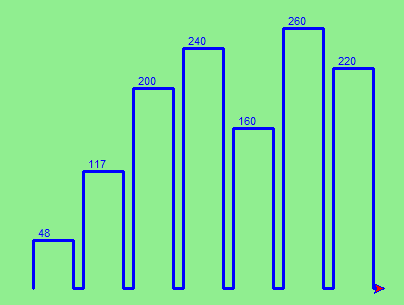
And now we'll add two lines to fill each bar. Our final program now looks like this:
def draw_bar(t, height):
    """ Get turtle t to draw one bar, of height. """
    t.begin_fill()           # Added this line
    t.left(90)
    t.forward(height)
    t.write("  "+ str(height))
    t.right(90)
    t.forward(40)
    t.right(90)
    t.forward(height)
    t.left(90)
    t.end_fill()             # Added this line
    t.forward(10)

wn = turtle.Screen()         # Set up the window and its attributes
wn.bgcolor("lightgreen")

tess = turtle.Turtle()       # Create tess and set some attributes
tess.color("blue", "red")
tess.pensize(3)

xs = [48,117,200,240,160,260,220]

for a in xs:
    draw_bar(tess, a)

wn.mainloop()
It produces the following, which is more satisfying:
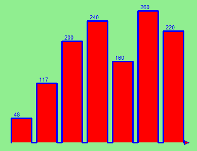
Mmm. Perhaps the bars should not be joined to each other at the bottom. We'll need to pick up the pen while making the gap between the bars. We'll leave that as an exercise for you!
Help and meta-notation
Python comes with extensive documentation for all its built-in functions, and its libraries.
The first source information is the website of Python itself. For the version of Python we are using, this documentation can be found on https://docs.python.org/3/. For instance, the documentation of the range function can be found here: https://docs.python.org/3/library/stdtypes.html#typesseq-range.
Notice the square brackets in the description of the arguments. These are examples of meta-notation --- notation that describes Python syntax, but is not part of it. The square brackets in this documentation mean that the argument is optional --- the programmer can omit it. So what this first line of help tells us is that range must always have a stop argument, but it may have an optional start argument (which must be followed by a comma if it is present), and it can also have an optional step argument, preceded by a comma if it is present.
The examples show that range can have either 1, 2 or 3 arguments. The list can start at any starting value, and go up or down in increments other than 1. The documentation here also says that the arguments must be integers.
Other meta-notation you'll frequently encounter is the use of bold and italics. The bold means that these are tokens --- keywords or symbols --- typed into your Python code exactly as they are, whereas the italic terms stand for "something of this type". So the syntax description
for variable in list :
means you can substitute any legal variable and any legal list when you write your Python code.
Towards encapsulation and generalization
In the end, most of the programs we write consist of functions. However, decomposing a program into functions is not an easy task. In the following sections we give another elaborate example to illustrate how to write a program that consists of functions. To this aim, we will start to write a program without functions, which we will subsequently improve afterwards.
In this example, we are interested in creating tables. Before computers were readily available, people had to calculate logarithms, sines and cosines, and other mathematical functions by hand. To make that easier, mathematics books contained long tables listing the values of these functions. Creating the tables was slow and boring, and they tended to be full of errors.
When computers appeared on the scene, one of the initial reactions was, "This is great! We can use the computers to generate the tables, so there will be no errors." That turned out to be true (mostly) but shortsighted. Soon thereafter, computers and calculators were so pervasive that the tables became obsolete.
Well, almost. For some operations, computers use tables of values to get an approximate answer and then perform computations to improve the approximation. In some cases, there have been errors in the underlying tables, most famously in the table the Intel Pentium processor chip used to perform floating-point division.
Although a log table is not as useful as it once was, it still makes a good example. The following program outputs a sequence of values in the left column and 2 raised to the power of that value in the right column:
for x in range(13):   # Generate numbers 0 to 12
    print(x, "\t", 2**x)
The string "\t" represents a tab character. The backslash character in "\t" indicates the beginning of an escape sequence. Escape sequences are used to represent invisible characters like tabs and newlines. The sequence \n represents a newline.
An escape sequence can appear anywhere in a string; in this example, the tab escape sequence is the only thing in the string.
As characters and strings are displayed on the screen, an invisible marker called the cursor keeps track of where the next character will go. After a print function, the cursor normally goes to the beginning of the next line.
The tab character shifts the cursor to the right until it reaches one of the tab stops. Tabs are useful for making columns of text line up, as in the output of the previous program:
0       1
1       2
2       4
3       8
4       16
5       32
6       64
7       128
8       256
9       512
10      1024
11      2048
12      4096
Because of the tab characters between the columns, the position of the second column does not depend on the number of digits in the first column.
Two-dimensional tables
Let's now make our example a little more complex.
A two-dimensional table is a table where you read the value at the intersection of a row and a column. A multiplication table is a good example. Let's say you want to print a multiplication table for the values from 1 to 6.
A good way to start is to write a loop that prints the multiples of 2, all on one line:
for i in range(6):
    print(2 * (i+1), end="   ")
print()
Here we've used the range function. As the loop executes, the value of i changes from 0 to 5. When all the elements of the range have been assigned to i, the loop terminates. Each time through the loop, it displays the value of 2 * i, followed by three spaces.
Again, the extra end=" " argument in the print function suppresses the newline, and uses three spaces instead. After the loop completes, the call to print at line 3 finishes the current line, and starts a new line.
The output of the program is:
2 4 6 8 10 12
So far, so good. We now have some pieces of code that we wish to put in functions. The next step is to encapsulate and generalize.
Encapsulation and generalization
Encapsulation is the process of wrapping a piece of code in a function, allowing you to take advantage of all the things functions are good for.
Generalization means taking something specific, such as printing the multiples of 2, and making it more general, such as printing the multiples of any integer.
This function encapsulates the previous loop and generalizes it to print multiples of n:
def print_multiples(n):
    for i in range(6):
        print(n * (i+1), end="   ")
    print()
To encapsulate, all we had to do was add the first line, which declares the name of the function and the parameter list. To generalize, all we had to do was replace the value 2 with the parameter n.
If we call this function with the argument 2, we get the same output as before. With the argument 3, the output is:
3 6 9 12 15 18
With the argument 4, the output is:
4 8 12 16 20 24
By now you can probably guess how to print a multiplication table --- by calling print_multiples repeatedly with different arguments. In fact, we can use another loop:
for i in range(6):
    print_multiples(i+1)
Notice how similar this loop is to the one inside print_multiples. All we did was replace the print function with a function call.
The output of this program is a multiplication table:
1      2      3      4      5      6
2      4      6      8      10     12
3      6      9      12     15     18
4      8      12     16     20     24
5      10     15     20     25     30
6      12     18     24     30     36
More encapsulation
To demonstrate encapsulation again, let's take the code from the last section and wrap it up in a function:
def print_mult_table():
    for i in range(6):
        print_multiples(i+1)
This process is a common development plan. We develop code by writing lines of code outside any function, or typing them in to the interpreter. When we get the code working, we extract it and wrap it up in a function.
This development plan is particularly useful if you don't know how to divide the program into functions when you start writing. This approach lets you design as you go along.
Local variables
You might be wondering how we can use the same variable, i, in both print_multiples and print_mult_table. Doesn't it cause problems when one of the functions changes the value of the variable?
The answer is no, because the i in print_multiples and the i in print_mult_table are not the same variable.
Variables created inside a function definition are local; you can't access a local variable from outside its home function. That means you are free to have multiple variables with the same name as long as they are not in the same function.
Python examines all the statements in a function --- if any of them assign a value to a variable, that is the clue that Python uses to make the variable a local variable.
The stack diagram for this program shows that the two variables named i are not the same variable. They can refer to different values, and changing one does not affect the other.
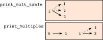
The value of i in print_mult_table goes from 1 to 6. In the diagram it happens to be 3. The next time through the loop it will be 4. Each time through the loop, print_mult_table calls print_multiples with the current value of i as an argument. That value gets assigned to the parameter n.
Inside print_multiples, the value of i goes from 1 to 6. In the diagram, it happens to be 2. Changing this variable has no effect on the value of i in print_mult_table.
It is common and perfectly legal to have different local variables with the same name. In particular, names like i and j are used frequently as loop variables. If you avoid using them in one function just because you used them somewhere else, you will probably make the program harder to read.
The visualizer at http://www.pythontutor.com/visualize.html shows very clearly how the two variables i are distinct variables, and how they have independent values.
More generalization
As another example of generalization, imagine you wanted a program that would print a multiplication table of any size, not just the six-by-six table. You could add a parameter to print_mult_table:
def print_mult_table(high):
    for i in range(high):
        print_multiples(i+1)
We replaced the value 6 with the expression high. If we call print_mult_table with the argument 7, it displays:
1      2      3      4      5      6
2      4      6      8      10     12
3      6      9      12     15     18
4      8      12     16     20     24
5      10     15     20     25     30
6      12     18     24     30     36
7      14     21     28     35     42
This is fine, except that we probably want the table to be square --- with the same number of rows and columns. To do that, we add another parameter to print_multiples to specify how many columns the table should have.
Just to be annoying, we call this parameter high, demonstrating that different functions can have parameters with the same name (just like local variables). Here's the whole program:
def print_multiples(n, high):
    for i in range(high):
        print(n * (i+1), end="   ")
    print()

def print_mult_table(high):
    for i in range(high):
        print_multiples(i+1, high)
Notice that when we added a new parameter, we had to change the first line of the function (the function heading), and we also had to change the place where the function is called in print_mult_table.
Now, when we call print_mult_table(7):
1      2      3      4      5      6      7
2      4      6      8      10     12     14
3      6      9      12     15     18     21
4      8      12     16     20     24     28
5      10     15     20     25     30     35
6      12     18     24     30     36     42
7      14     21     28     35     42     49
When you generalize a function appropriately, you often get a program with capabilities you didn't plan. For example, you might notice that, because ab = ba, all the entries in the table appear twice. You could save ink by printing only half the table. To do that, you only have to change one line of print_mult_table. Change
print_multiples(i, high)
to
print_multiples(i, i)
and you get:
1
2      4
3      6      9
4      8      12     16
5      10     15     20     25
6      12     18     24     30     36
7      14     21     28     35     42     49
Functions
A few times now, we have mentioned all the things functions are good for. Let's summarize this:
- Capturing your mental chunking. Breaking your complex tasks into sub-tasks, and giving the sub-tasks a meaningful name is a powerful mental technique. Look back at the example that illustrated the post-test loop: we assumed that we had a function called play_the_game_once. This chunking allowed us to put aside the details of the particular game --- is it a card game, or noughts and crosses, or a role playing game --- and simply focus on one isolated part of our program logic --- letting the player choose whether they want to play again.
- Dividing a long program into functions allows you to separate parts of the program, debug them in isolation, and then compose them into a whole.
- Functions facilitate the use of iteration.
- Well-designed functions are often useful for many programs. Once you write and debug one, you can reuse it.
Glossary
- argument
- A value provided to a function when the function is called. This value is assigned to the corresponding parameter in the function. The argument can be the result of an expression which may involve operators, operands and calls to other fruitful functions.
- body
- The second part of a compound statement. The body consists of a sequence of statements all indented the same amount from the beginning of the header. The standard amount of indentation used within the Python community is 4 spaces.
- compound statement
A statement that consists of two parts:
- header - which begins with a keyword determining the statement type, and ends with a colon.
- body - containing one or more statements indented the same amount from the header.
The syntax of a compound statement looks like this:
keyword ... : statement statement ...- docstring
- A special string that is attached to a function as its __doc__ attribute. Tools can use docstrings to provide documentation or hints for the programmer. When we get to modules, classes, and methods, we'll see that docstrings can also be used there.
- flow of execution
- The order in which statements are executed during a program run.
- frame
- A box in a stack diagram that represents a function call. It contains the local variables and parameters of the function.
- function
- A named sequence of statements that performs some useful operation. Functions may or may not take parameters and may or may not produce a result.
- function call
- A statement that executes a function. It consists of the name of the function followed by a list of arguments enclosed in parentheses.
- function composition
- Using the output from one function call as the input to another.
- function definition
- A statement that creates a new function, specifying its name, parameters, and the statements it executes.
- fruitful function
- A function that returns a value when it is called.
- header line
- The first part of a compound statement. A header line begins with a keyword and ends with a colon (:)
- import statement
- A statement which permits functions and variables defined in another Python module to be brought into the environment of another script. To use the features of the turtle, we need to first import the turtle module.
- lifetime
- Variables and objects have lifetimes --- they are created at some point during program execution, and will be destroyed at some time.
- local variable
- A variable defined inside a function. A local variable can only be used inside its function. Parameters of a function are also a special kind of local variable.
- parameter
- A name used inside a function to refer to the value which was passed to it as an argument.
- refactor
- A fancy word to describe reorganizing our program code, usually to make it more understandable. Typically, we have a program that is already working, then we go back to "tidy it up". It often involves choosing better variable names, or spotting repeated patterns and moving that code into a function.
- stack diagram
- A graphical representation of a stack of functions, their variables, and the values to which they refer.
- traceback
- A list of the functions that are executing, printed when a runtime error occurs. A traceback is also commonly refered to as a stack trace, since it lists the functions in the order in which they are stored in the runtime stack.
- void function
- The opposite of a fruitful function: one that does not return a value. It is executed for the work it does, rather than for the value it returns.
References
| [ThinkCS] | How To Think Like a Computer Scientist --- Learning with Python 3 |
Fruitful functions
Source: this section is heavily based on Chapter 6 of [ThinkCS].
Return values
The built-in functions we have used, such as abs, pow, int, max, and range, have produced results. Calling each of these functions generates a value, which we usually assign to a variable or use as part of an expression.
biggest = max(3, 7, 2, 5)
x = abs(3 - 11) + 10
We also wrote our own function to return the final amount for a compound interest calculation.
In this chapter, we are going to write more functions that return values, which we will call fruitful functions, for want of a better name. The first example is area, which returns the area of a circle with the given radius:
def area(radius):
    b = 3.14159 * radius**2
    return b
We have seen the return statement before, but in a fruitful function the return statement includes a return value. This statement means: evaluate the return expression, and then return it immediately as the result (the fruit) of this function. The expression provided can be arbitrarily complicated, so we could have written this function like this:
def area(radius):
    return 3.14159 * radius * radius
On the other hand, temporary variables like b above often make debugging easier.
Sometimes it is useful to have multiple return statements, one in each branch of a conditional. We have already seen the built-in abs, now we see how to write our own:
def absolute_value(x):
    if x < 0:
        return -x
    else:
        return x
Another way to write the above function is to leave out the else and just follow the if condition by the second return statement.
def absolute_value(x):
    if x < 0:
        return -x
    return x
Think about this version and convince yourself it works the same as the first one.
Code that appears after a return statement, or any other place the flow of execution can never reach, is called dead code, or unreachable code.
In a fruitful function, it is a good idea to ensure that every possible path through the program hits a return statement. The following version of absolute_value fails to do this:
def bad_absolute_value(x):
    if x < 0:
        return -x
    elif x > 0:
        return x
This version is not correct because if x happens to be 0, neither condition is true, and the function ends without hitting a return statement. In this case, the return value is a special value called None:
>>> print(bad_absolute_value(0))
None
All Python functions return None whenever they do not return another value.
It is also possible to use a return statement in the middle of a for loop, in which case control immediately returns from the function. Let us assume that we want a function which looks through a list of words. It should return the first 2-letter word. If there is not one, it should return the empty string:
def find_first_2_letter_word(xs):
    for wd in xs:
        if len(wd) == 2:
           return wd
    return ""
>>> find_first_2_letter_word(["This", "is", "a", "dead", "parrot"]) 'is' >>> find_first_2_letter_word(["I", "like", "cheese"]) ''
Single-step through this code and convince yourself that in the first test case that we've provided, the function returns while processing the second element in the list: it does not have to traverse the whole list.
Return vs print
The purpose of a fruitful function is to do a calculation, the result of which is used later in another part of the program; as we have seen now, return is used to return a value to the rest of the program.
However, in earlier chapters, we have often used functions such as print and input. For instance, we wrote:
n = int(input("Give a number: "))
count = 0
while n > 0:
    count = count + 1
    n = n // 10
print(count)
Is the difference with the following code really important?
def ndigits ( n ):
    count = 0
    while n > 0:
        count = count + 1
        n = n // 10
    return count
Unfortunately, this difference is extremely important. Most functions are supposed to interact with the rest of the program, and not with the user. In this case, we should use return, and not print.
At the exam, we will (almost) always ask to write programs that interact with our evaluation system, not with some hypothetical user. Hence, if at the exam we ask you to write a function that returns the number of digits in the decimal representation of an integer, code without return is absolutely incorrect; you will not get any points for it! Similarly, the following answers are all incorrect:
def ndigits ( n ):
    n = int(input("Give a number: "))
    count = 0
    while n > 0:
        count = count + 1
        n = n // 10
    print(count)

def ndigits ( n ):
    count = 0
    while n > 0:
        count = count + 1
        n = n // 10
    print(count)
The core problem with these implementations is that input and print are functions that interact with the user, but not with the rest of the program. In all functions that use print, print will display the result of the calculation on the screen, but it will not provide this result to the rest of the program. If at the exam the rest of this program has to calculate a grade for your answer, without return it has nothing to work on!!!
Hence, be very careful with the use of print; when writing functions, you will need return most of the times.
Program development
At this point, you should be able to look at complete functions and tell what they do. Also, if you have been doing the exercises, you have written some small functions. As you write larger functions, you might start to have more difficulty, especially with runtime and semantic errors.
To deal with increasingly complex programs, we are going to suggest a technique called incremental development. The goal of incremental development is to avoid long debugging sessions by adding and testing only a small amount of code at a time.
As an example, suppose we want to find the distance between two points, given by the coordinates (x1, y1) and (x2, y2). By the Pythagorean theorem, the distance is:
The first step is to consider what a distance function should look like in Python. In other words, what are the inputs (parameters) and what is the output (return value)?
In this case, the two points are the inputs, which we can represent using four parameters. The return value is the distance, which is a floating-point value.
Already we can write an outline of the function that captures our thinking so far:
def distance(x1, y1, x2, y2):
    return 0.0
Obviously, this version of the function doesn't compute distances; it always returns zero. But it is syntactically correct, and it will run, which means that we can test it before we make it more complicated.
To test the new function, we call it with sample values:
>>> distance(1, 2, 4, 6)
0.0
We chose these values so that the horizontal distance equals 3 and the vertical distance equals 4; that way, the result is 5 (the hypotenuse of a 3-4-5 triangle). When testing a function, it is useful to know the right answer.
At this point we have confirmed that the function is syntactically correct, and we can start adding lines of code. After each incremental change, we test the function again. If an error occurs at any point, we know where it must be --- in the last line we added.
A logical first step in the computation is to find the differences x2- x1 and y2- y1. We will refer to those values using temporary variables named dx and dy.
def distance(x1, y1, x2, y2):
    dx = x2 - x1
    dy = y2 - y1
    return 0.0
If we call the function with the arguments shown above, when the flow of execution gets to the return statement, dx should be 3 and dy should be 4. We can check that this is the case in Thonny by putting the cursor on the return statement, and putting a breakpoint on that line. Then we inspect the variables dx and dy by hovering the mouse above them, to confirm that the function is getting the right parameters and performing the first computation correctly. If not, there are only a few lines to check.
Next we compute the sum of squares of dx and dy:
def distance(x1, y1, x2, y2):
    dx = x2 - x1
    dy = y2 - y1
    dsquared = dx*dx + dy*dy
    return 0.0
Again, we could run the program at this stage and check the value of dsquared (which should be 25).
Finally, using the fractional exponent 0.5 to find the square root, we compute and return the result:
def distance(x1, y1, x2, y2):
    dx = x2 - x1
    dy = y2 - y1
    dsquared = dx*dx + dy*dy
    result = dsquared**0.5
    return result
If that works correctly, you are done. Otherwise, you might want to inspect the value of result before the return statement.
When you start out, you might add only a line or two of code at a time. As you gain more experience, you might find yourself writing and debugging bigger conceptual chunks. Either way, stepping through your code one line at a time and verifying that each step matches your expectations can save you a lot of debugging time. As you improve your programming skills you should find yourself managing bigger and bigger chunks: this is very similar to the way we learned to read letters, syllables, words, phrases, sentences, paragraphs, etc., or the way we learn to chunk music --- from individual notes to chords, bars, phrases, and so on.
The key aspects of the process are:
- Start with a working skeleton program and make small incremental changes. At any point, if there is an error, you will know exactly where it is.
- Use temporary variables to refer to intermediate values so that you can easily inspect and check them.
- Once the program is working, relax, sit back, and play around with your options. (There is interesting research that links "playfulness" to better understanding, better learning, more enjoyment, and a more positive mindset about what you can achieve --- so spend some time fiddling around!) You might want to consolidate multiple statements into one bigger compound expression, or rename the variables you've used, or see if you can make the function shorter. A good guideline is to aim for making code as easy as possible for others to read.
Here is another version of the function. It makes use of a square root function that is in the math module (we'll learn about modules shortly). Which do you prefer? Which looks "closer" to the Pythagorean formula we started out with?
import math

def distance(x1, y1, x2, y2):
    return math.sqrt( (x2-x1)**2 + (y2-y1)**2 )
>>> distance(1, 2, 4, 6) 5.0
Debugging with print
Another powerful technique for debugging (an alternative to single-stepping and inspection of program variables), is to insert extra print functions in carefully selected places in your code. Then, by inspecting the output of the program, you can check whether the algorithm is doing what you expect it to. Be clear about the following, however:
You must have a clear solution to the problem, and must know what should happen before you can debug a program. Work on solving the problem on a piece of paper (perhaps using a flowchart to record the steps you take) before you concern yourself with writing code. Writing a program doesn't solve the problem --- it simply automates the manual steps you would take. So first make sure you have a pen-and-paper manual solution that works. Programming then is about making those manual steps happen automatically.
Do not write chatterbox functions. A chatterbox is a fruitful function that, in addition to its primary task, also asks the user for input, or prints output, when it would be more useful if it simply shut up and did its work quietly.
For example, we've seen built-in functions like range, max and abs. None of these would be useful building blocks for other programs if they prompted the user for input, or printed their results while they performed their tasks.
So we wish to repeat our statement earlier in this chapter: avoid calling print and input functions inside fruitful functions, unless the primary purpose of your function is to perform input and output. The one exception to this rule might be to temporarily sprinkle some calls to print into your code to help debug and understand what is happening when the code runs, but these will then be removed once you get things working; once more, also at the exam, these statements are not considered.
Composition
As you should expect by now, you can call one function from within another. This ability is called composition.
As an example, we'll write a function that takes two points, the center of the circle and a point on the perimeter, and computes the area of the circle.
Assume that the center point is stored in the variables xc and yc, and the perimeter point is in xp and yp. The first step is to find the radius of the circle, which is the distance between the two points. Fortunately, we've just written a function, distance, that does just that, so now all we have to do is use it:
radius = distance(xc, yc, xp, yp)
The second step is to find the area of a circle with that radius and return it. Again we will use one of our earlier functions:
result = area(radius)
return result
Wrapping that up in a function, we get:
def area2(xc, yc, xp, yp):
    radius = distance(xc, yc, xp, yp)
    result = area(radius)
    return result
We called this function area2 to distinguish it from the area function defined earlier.
The temporary variables radius and result are useful for development, debugging, and single-stepping through the code to inspect what is happening, but once the program is working, we can make it more concise by composing the function calls:
def area2(xc, yc, xp, yp):
    return area(distance(xc, yc, xp, yp))
Boolean functions
Functions can return Boolean values, which is often convenient for hiding complicated tests inside functions. For example:
def is_divisible(x, y):
    """ Test if x is exactly divisible by y """
    if x % y == 0:
        return True
    else:
        return False
It is common to give Boolean functions names that sound like yes/no questions. is_divisible returns either True or False to indicate whether the x is or is not divisible by y.
We can make the function more concise by taking advantage of the fact that the condition of the if statement is itself a Boolean expression. We can return it directly, avoiding the if statement altogether:
def is_divisible(x, y):
    return x % y == 0
This session shows the new function in action:
>>> is_divisible(6, 4)
False
>>> is_divisible(6, 3)
True
Boolean functions are often used in conditional statements:
if is_divisible(x, y):
    ... # Do something ...
else:
    ... # Do something else ...
It might be tempting to write something like:
if is_divisible(x, y) == True:
but the extra comparison is unnecessary.
Programming with style
Readability is very important to programmers, since in practice programs are read and modified far more often then they are written. But, like most rules, we occasionaly break them. Most of the code examples in this book will be consistent with the Python Enhancement Proposal 8 (PEP 8), a style guide developed by the Python community.
We'll have more to say about style as our programs become more complex, but a few pointers will be helpful already:
- use 4 spaces (instead of tabs) for indentation
- limit line length to 78 characters
- when naming identifiers, use CamelCase for classes (we'll get to those) and lowercase_with_underscores for functons and variables
- place imports at the top of the file
- keep function definitions together
- use docstrings to document functions
- use two blank lines to separate function definitions from each other
- keep top level statements, including function calls, together at the bottom of the program
Unit testing
It is a common best practice in software development to include automatic unit testing of source code. Unit testing provides a way to automatically verify that individual pieces of code, such as functions, are working properly. This makes it possible to change the implementation of a function at a later time and quickly test that it still does what it was intended to do.
Some years back organizations had the view that their valuable asset was the program code and documentation. Organizations will now spend a large portion of their software budgets on crafting (and preserving) their tests.
Unit testing also forces the programmer to think about the different cases that the function needs to handle. You also only have to type the tests once into the script, rather than having to keep entering the same test data over and over as you develop your code.
Extra code in your program which is there because it makes debugging or testing easier is called scaffolding.
A collection of tests for some code is called its test suite.
There are a few different ways to do unit testing in Python --- but at this stage we're going to ignore what the Python community usually does, and we're going to start with two functions that we'll write ourselves. We'll use these for writing our unit tests.
Let's start with the absolute_value function that we wrote earlier in this chapter. Recall that we wrote a few different versions, the last of which was incorrect, and had a bug. Would tests have caught this bug?
First we plan our tests. We'd like to know if the function returns the correct value when its argument is negative, or when its argument is positive, or when its argument is zero. When planning your tests, you'll always want to think carefully about the "edge" cases --- here, an argument of 0 to absolute_value is on the edge of where the function behaviour changes, and as we saw at the beginning of the chapter, it is an easy spot for the programmer to make a mistake! So it is a good case to include in our test suite.
We're going to write a helper function for checking the results of one test. It takes a boolean argument and will either print a message telling us that the test passed, or it will print a message to inform us that the test failed. The first line of the body (after the function's docstring) magically determines the line number in the script where the call was made from. This allows us to print the line number of the test, which will help when we want to identify which tests have passed or failed.
import sys

def test(did_pass):
    """  Print the result of a test.  """
    linenum = sys._getframe(1).f_lineno   # Get the caller's line number.
    if did_pass:
        msg = "Test at line {0} ok.".format(linenum)
    else:
        msg = ("Test at line {0} FAILED.".format(linenum))
    print(msg)
There is also some slightly tricky string formatting using the format method which we will gloss over for the moment, and cover in detail in a future chapter. But with this function written, we can proceed to construct our test suite:
def test_suite():
    """ Run the suite of tests for code in this module (this file).
    """
    test(absolute_value(17) == 17)
    test(absolute_value(-17) == 17)
    test(absolute_value(0) == 0)
    test(absolute_value(3.14) == 3.14)
    test(absolute_value(-3.14) == 3.14)

test_suite()        # Here is the call to run the tests
Here you'll see that we've constructed five tests in our test suite. We could run this against the first or second versions (the correct versions) of absolute_value, and we'd get output similar to the following:
Test at line 25 ok.
Test at line 26 ok.
Test at line 27 ok.
Test at line 28 ok.
Test at line 29 ok.
But let's say you change the function to an incorrect version like this:
def absolute_value(n):   # Buggy version
    """ Compute the absolute value of n """
    if n < 0:
        return 1
    elif n > 0:
        return n
Can you find at least two mistakes in this code? Our test suite can! We get:
Test at line 25 ok.
Test at line 26 FAILED.
Test at line 27 FAILED.
Test at line 28 ok.
Test at line 29 FAILED.
These are three examples of failing tests.
There is a built-in Python statement called assert that does almost the same as our test function (except the program stops when the first assertion fails). You may want to read about it, and use it instead of our test function.
The early return
The return statement, with or without a value, depending on whether the function is fruitful or void, allows us to terminate the execution of a function before (or when) we reach the end. One reason to use an early return is if we detect an error condition:
def print_square_root(x):
    if x <= 0:
        print("Positive numbers only, please.")
        return

    result = x**0.5
    print("The square root of", x, "is", result)
The function print_square_root has a parameter named x. The first thing it does is check whether x is less than or equal to 0, in which case it displays an error message and then uses return to exit the function. The flow of execution immediately returns to the caller, and the remaining lines of the function are not executed.
Glossary
- Boolean function
- A function that returns a Boolean value. The only possible values of the bool type are False and True.
- chatterbox function
- A function which interacts with the user (using input or print) when it should not. Silent functions that just convert their input arguments into their output results are usually the most useful ones.
- composition (of functions)
- Calling one function from within the body of another, or using the return value of one function as an argument to the call of another.
- dead code
- Part of a program that can never be executed, often because it appears after a return statement.
- fruitful function
- A function that yields a return value instead of None.
- incremental development
- A program development plan intended to simplify debugging by adding and testing only a small amount of code at a time.
- None
- A special Python value. One use in Python is that it is returned by functions that do not execute a return statement with a return argument.
- return value
- The value provided as the result of a function call.
- scaffolding
- Code that is used during program development to assist with development and debugging. The unit test code that we added in this chapter are examples of scaffolding.
- temporary variable
- A variable used to store an intermediate value in a complex calculation.
- test suite
- A collection of tests for some code you have written.
- unit testing
- An automatic procedure used to validate that individual units of code are working properly. Having a test suite is extremely useful when somebody modifies or extends the code: it provides a safety net against going backwards by putting new bugs into previously working code. The term regression testing is often used to capture this idea that we don't want to go backwards!
- wrapping code in a function
- The process of adding a function header and parameters to a sequence of program statements is often refered to as "wrapping the code in a function". This process is very useful whenever the program statements in question are going to be used multiple times. It is even more useful when it allows the programmer to express their mental chunking, and how they've broken a complex problem into pieces.
References
| [ThinkCS] | How To Think Like a Computer Scientist --- Learning with Python 3 |
Modules
Source: this section is heavily based on Chapter 12 of [ThinkCS].
A module is a file containing Python definitions and statements intended for use in other Python programs. There are many Python modules that come with Python as part of the standard library. We have seen at least two of these already, the turtle module and the string module.
We have also shown you how to access help. The help system contains a listing of all the standard modules that are available with Python. Play with help!
Random numbers
We often want to use random numbers in programs, here are a few typical uses:
- To play a game of chance where the computer needs to throw some dice, pick a number, or flip a coin,
- To shuffle a deck of playing cards randomly,
- To allow/make an enemy spaceship appear at a random location and start shooting at the player,
- To simulate possible rainfall when we make a computerized model for estimating the environmental impact of building a dam,
- For encrypting banking sessions on the Internet.
Python provides a module random that helps with tasks like this. You can look it up using help, but here are the key things we'll do with it:
import random

# Create a black box object that generates random numbers
rng = random.Random()

dice_throw = rng.randrange(1,7)   # Return an int, one of 1,2,3,4,5,6
delay_in_seconds = rng.random() * 5.0
The randrange method call generates an integer between its lower and upper argument, using the same semantics as range --- so the lower bound is included, but the upper bound is excluded. All the values have an equal probability of occurring (i.e. the results are uniformly distributed). Like range, randrange can also take an optional step argument. So let's assume we needed a random odd number less than 100, we could say:
r_odd = rng.randrange(1, 100, 2)
Other methods can also generate other distributions e.g. a bell-shaped, or "normal" distribution might be more appropriate for estimating seasonal rainfall, or the concentration of a compound in the body after taking a dose of medicine.
The random method returns a floating point number in the interval [0.0, 1.0) --- the square bracket means "closed interval on the left" and the round parenthesis means "open interval on the right". In other words, 0.0 is possible, but all returned numbers will be strictly less than 1.0. It is usual to scale the results after calling this method, to get them into an interval suitable for your application. In the case shown here, we've converted the result of the method call to a number in the interval [0.0, 5.0). Once more, these are uniformly distributed numbers --- numbers close to 0 are just as likely to occur as numbers close to 0.5, or numbers close to 1.0.
This example shows how to shuffle a list. (shuffle cannot work directly with a lazy promise, so notice that we had to convert the range object using the list type converter first.)
cards = list(range(52))  # Generate ints [0 .. 51]
                         #    representing a pack of cards.
rng.shuffle(cards)       # Shuffle the pack
Repeatability and Testing
Random number generators are based on a deterministic algorithm --- repeatable and predictable. So they're called pseudo-random generators --- they are not genuinely random. They start with a seed value. Each time you ask for another random number, you'll get one based on the current seed attribute, and the state of the seed (which is one of the attributes of the generator) will be updated.
For debugging and for writing unit tests, it is convenient to have repeatability --- programs that do the same thing every time they are run. We can arrange this by forcing the random number generator to be initialized with a known seed every time. (Often this is only wanted during testing --- playing a game of cards where the shuffled deck was always in the same order as last time you played would get boring very rapidly!)
drng = random.Random(123) # Create generator with known starting state
This alternative way of creating a random number generator gives an explicit seed value to the object. Without this argument, the system probably uses something based on the time. So grabbing some random numbers from drng today will give you precisely the same random sequence as it will tomorrow!
Picking balls from bags, throwing dice, shuffling a pack of cards
Here is an example to generate a list containing n random ints between a lower and an upper bound:
import random

def make_random_ints(num, lower_bound, upper_bound):
   """
     Generate a list containing num random ints between lower_bound
     and upper_bound. upper_bound is an open bound.
   """
   rng = random.Random()  # Create a random number generator
   result = []
   for i in range(num):
      result.append(rng.randrange(lower_bound, upper_bound))
   return result
>>> make_random_ints(5, 1, 13) # Pick 5 random month numbers [8, 1, 8, 5, 6]
Notice that we got a duplicate in the result. Often this is wanted, e.g. if we throw a die five times, we would expect some duplicates.
But what if you don't want duplicates? If you wanted 5 distinct months, then this algorithm is wrong. In this case a good algorithm is to generate the list of possibilities, shuffle it, and slice off the number of elements you want:
xs = list(range(1,13))  # Make list 1..12  (there are no duplicates)
rng = random.Random()   # Make a random number generator
rng.shuffle(xs)         # Shuffle the list
result = xs[:5]         # Take the first five elements
In statistics courses, the first case --- allowing duplicates --- is usually described as pulling balls out of a bag with replacement --- you put the drawn ball back in each time, so it can occur again. The latter case, with no duplicates, is usually described as pulling balls out of the bag without replacement. Once the ball is drawn, it doesn't go back to be drawn again. TV lotto games work like this.
The second "shuffle and slice" algorithm would not be so great if you only wanted a few elements, but from a very large domain. Suppose I wanted five numbers between one and ten million, without duplicates. Generating a list of ten million items, shuffling it, and then slicing off the first five would be a performance disaster! So let us have another try:
import random

def make_random_ints_no_dups(num, lower_bound, upper_bound):
   """
     Generate a list containing num random ints between
     lower_bound and upper_bound. upper_bound is an open bound.
     The result list cannot contain duplicates.
   """
   result = []
   rng = random.Random()
   for i in range(num):
        while True:
            candidate = rng.randrange(lower_bound, upper_bound)
            if candidate not in result:
                break
        result.append(candidate)
   return result

xs = make_random_ints_no_dups(5, 1, 10000000)
print(xs)
This agreeably produces 5 random numbers, without duplicates:
[3344629, 1735163, 9433892, 1081511, 4923270]
Even this function has its pitfalls. Can you spot what is going to happen in this case?
xs = make_random_ints_no_dups(10, 1, 6)
The time module
As we start to work with more sophisticated algorithms and bigger programs, a natural concern is "is our code efficient?" One way to experiment is to time how long various operations take. The time module has a function called clock that is recommended for this purpose. Whenever clock is called, it returns a floating point number representing how many seconds have elapsed since your program started running.
The way to use it is to call clock and assign the result to a variable, say t0, just before you start executing the code you want to measure. Then after execution, call clock again, (this time we'll save the result in variable t1). The difference t1-t0 is the time elapsed, and is a measure of how fast your program is running.
Let's try a small example. Python has a built-in sum function that can sum the elements in a list. We can also write our own. How do we think they would compare for speed? We'll try to do the summation of a list [0, 1, 2 ...] in both cases, and compare the results:
import time

def do_my_sum(xs):
    sum = 0
    for v in xs:
        sum += v
    return sum

sz = 10000000        # Lets have 10 million elements in the list
testdata = range(sz)

t0 = time.clock()
my_result = do_my_sum(testdata)
t1 = time.clock()
print("my_result    = {0} (time taken = {1:.4f} seconds)"
        .format(my_result, t1-t0))

t2 = time.clock()
their_result = sum(testdata)
t3 = time.clock()
print("their_result = {0} (time taken = {1:.4f} seconds)"
        .format(their_result, t3-t2))
On a reasonably modest laptop, we get these results:
my_sum    = 49999995000000 (time taken = 1.5567 seconds)
their_sum = 49999995000000 (time taken = 0.9897 seconds)
So our function runs about 57% slower than the built-in one. Generating and summing up ten million elements in under a second is not too shabby!
The math module
The math module contains the kinds of mathematical functions you'd typically find on your calculator (sin, cos, sqrt, asin, log, log10) and some mathematical constants like pi and e:
>>> import math
>>> math.pi                 # Constant pi
3.141592653589793
>>> math.e                  # Constant natural log base
2.718281828459045
>>> math.sqrt(2.0)          # Square root function
1.4142135623730951
>>> math.radians(90)        # Convert 90 degrees to radians
1.5707963267948966
>>> math.sin(math.radians(90))  # Find sin of 90 degrees
1.0
>>> math.asin(1.0) * 2      # Double the arcsin of 1.0 to get pi
3.141592653589793
Like almost all other programming languages, angles are expressed in radians rather than degrees. There are two functions radians and degrees to convert between these two popular ways of measuring angles.
Notice another difference between this module and our use of random and turtle: in random and turtle we create objects and we call methods on the object. This is because objects have state --- a turtle has a color, a position, a heading, etc., and every random number generator has a seed value that determines its next result.
Mathematical functions are "pure" and don't have any state --- calculating the square root of 2.0 doesn't depend on any kind of state or history about what happened in the past. So the functions are not methods of an object --- they are simply functions that are grouped together in a module called math.
Creating your own modules
All we need to do to create our own modules is to save our script as a file with a .py extension. Suppose, for example, this script is saved as a file named seqtools.py:
def remove_at(pos, seq):
    return seq[:pos] + seq[pos+1:]
We can now use our module, both in scripts we write, or in the interactive Python interpreter. To do so, we must first import the module.
>>> import seqtools
>>> s = "A string!"
>>> seqtools.remove_at(4, s)
'A sting!'
We do not include the .py file extension when importing. Python expects the file names of Python modules to end in .py, so the file extension is not included in the import statement.
The use of modules makes it possible to break up very large programs into manageable sized parts, and to keep related parts together.
Namespaces
A namespace is a collection of identifiers that belong to a module, or to a function, (and as we will see soon, in classes too). Generally, we like a namespace to hold "related" things, e.g. all the math functions, or all the typical things we'd do with random numbers.
Each module has its own namespace, so we can use the same identifier name in multiple modules without causing an identification problem.
# Module1.py

question = "What is the meaning of Life, the Universe, and Everything?"
answer = 42
# Module2.py question = "What is your quest?" answer = "To seek the holy grail."
We can now import both modules and access question and answer in each:
import module1
import module2

print(module1.question)
print(module2.question)
print(module1.answer)
print(module2.answer)
will output the following:
What is the meaning of Life, the Universe, and Everything?
What is your quest?
42
To seek the holy grail.
Functions also have their own namespaces:
def f():
    n = 7
    print("printing n inside of f:", n)

def g():
    n = 42
    print("printing n inside of g:", n)

n = 11
print("printing n before calling f:", n)
f()
print("printing n after calling f:", n)
g()
print("printing n after calling g:", n)
Running this program produces the following output:
printing n before calling f: 11
printing n inside of f: 7
printing n after calling f: 11
printing n inside of g: 42
printing n after calling g: 11
The three n's here do not collide since they are each in a different namespace --- they are three names for three different variables, just like there might be three different instances of people, all called "Bruce".
Namespaces permit several programmers to work on the same project without having naming collisions.
Scope and lookup rules
The scope of an identifier is the region of program code in which the identifier can be accessed, or used.
There are three important scopes in Python:
- Local scope refers to identifiers declared within a function. These identifiers are kept in the namespace that belongs to the function, and each function has its own namespace.
- Global scope refers to all the identifiers declared within the current module, or file.
- Built-in scope refers to all the identifiers built into Python --- those like range and min that can be used without having to import anything, and are (almost) always available.
Python (like most other computer languages) uses precedence rules: the same name could occur in more than one of these scopes, but the innermost, or local scope, will always take precedence over the global scope, and the global scope always gets used in preference to the built-in scope. Let's start with a simple example:
def range(n):
    return 123*n

print(range(10))
What gets printed? We've defined our own function called range, so there is now a potential ambiguity. When we use range, do we mean our own one, or the built-in one? Using the scope lookup rules determines this: our own range function, not the built-in one, is called, because our function range is in the global namespace, which takes precedence over the built-in names.
So although names likes range and min are built-in, they can be "hidden" from your use if you choose to define your own variables or functions that reuse those names. (It is a confusing practice to redefine built-in names --- so to be a good programmer you need to understand the scope rules and understand that you can do nasty things that will cause confusion, and then you avoid doing them!)
Now, a slightly more complex example:
n = 10
m = 3
def f(n):
   m = 7
   return 2*n+m

print(f(5), n, m)
This prints 17 10 3. The reason is that the two variables m and n in lines 1 and 2 are outside the function in the global namespace. Inside the function, new variables called n and m are created just for the duration of the execution of f. These are created in the local namespace of function f. Within the body of f, the scope lookup rules determine that we use the local variables m and n. By contrast, after we've returned from f, the n and m arguments to the print function refer to the original variables on lines 1 and 2, and these have not been changed in any way by executing function f.
Notice too that the def puts name f into the global namespace here. So it can be called on line 7.
What is the scope of the variable n on line 1? Its scope --- the region in which it is visible --- is lines 1, 2, 6, 7. It is hidden from view in lines 3, 4, 5 because of the local variable n.
Attributes and the dot operator
Variables defined inside a module are called attributes of the module. We've seen that objects have attributes too: for example, most objects have a __doc__ attribute, some functions have a __annotations__ attribute. Attributes are accessed using the dot operator (.). The question attribute of module1 and module2 is accessed using module1.question and module2.question.
Modules contain functions as well as attributes, and the dot operator is used to access them in the same way. seqtools.remove_at refers to the remove_at function in the seqtools module.
When we use a dotted name, we often refer to it as a fully qualified name, because we're saying exactly which question attribute we mean.
Three import statement variants
Here are three different ways to import names into the current namespace, and to use them:
import math
x = math.sqrt(10)
Here just the single identifier math is added to the current namespace. If you want to access one of the functions in the module, you need to use the dot notation to get to it.
Here is a different arrangement:
from math import cos, sin, sqrt
x = sqrt(10)
The names are added directly to the current namespace, and can be used without qualification. The name math is not itself imported, so trying to use the qualified form math.sqrt would give an error.
Then we have a convenient shorthand:
from math import *   # Import all the identifiers from math,
                     #   adding them to the current namespace.
x = sqrt(10)         # Use them without qualification.
Of these three, the first method is generally preferred, even though it means a little more typing each time. Although, we can make things shorter by importing a module under a different name:
>>> import math as m
>>> m.pi
3.141592653589793
But hey, with nice editors that do auto-completion, and fast fingers, that's a small price!
Finally, observe this case:
def area(radius):
    import math
    return math.pi * radius * radius

x = math.sqrt(10)      # This gives an error
Here we imported math, but we imported it into the local namespace of area. So the name is usable within the function body, but not in the enclosing script, because it is not in the global namespace.
Turn your unit tester into a module
Near the end of Chapter 6 (Fruitful functions) we introduced unit testing, and our own test function, and you've had to copy this into each module for which you wrote tests. Now we can put that definition into a module of its own, say unit_tester.py, and simply use one line in each new script instead:
from unit_tester import test
Glossary
- attribute
- A variable defined inside a module (or class or instance -- as we will see later). Module attributes are accessed by using the dot operator (.).
- dot operator
- The dot operator (.) permits access to attributes and functions of a module (or attributes and methods of a class or instance -- as we have seen elsewhere).
- fully qualified name
- A name that is prefixed by some namespace identifier and the dot operator, or by an instance object, e.g. math.sqrt or tess.forward(10).
- import statement
A statement which makes the objects contained in a module available for use within another module. There are two forms for the import statement. Using hypothetical modules named mymod1 and mymod2 each containing functions f1 and f2, and variables v1 and v2, examples of these two forms include:
import mymod1
from mymod2 import f1, f2, v1, v2
The second form brings the imported objects into the namespace of the importing module, while the first form preserves a separate namespace for the imported module, requiring mymod1.v1 to access the v1 variable from that module.
- method
Function-like attribute of an object. Methods are invoked (called) on an object using the dot operator. For example:
>>> s = "this is a string."
>>> s.upper()
'THIS IS A STRING.'
>>>
We say that the method, upper is invoked on the string, s. s is implicitely the first argument to upper.
- module
- A file containing Python definitions and statements intended for use in other Python programs. The contents of a module are made available to the other program by using the import statement.
- namespace
- A syntactic container providing a context for names so that the same name can reside in different namespaces without ambiguity. In Python, modules, classes, functions and methods all form namespaces.
- naming collision
A situation in which two or more names in a given namespace cannot be unambiguously resolved. Using
import stringinstead of
from string import *prevents naming collisions.
- standard library
- A library is a collection of software used as tools in the development of other software. The standard library of a programming language is the set of such tools that are distributed with the core programming language. Python comes with an extensive standard library.
References
| [ThinkCS] | How To Think Like a Computer Scientist --- Learning with Python 3 |
Table des matières
Data Structures
Strings
Source: this section is heavily based on Chapter 8 of [ThinkCS].
A compound data type
So far we have seen built-in types like int, float, bool, str and we've seen lists and pairs. Strings, lists, and pairs are qualitatively different from the others because they are made up of smaller pieces. In the case of strings, they're made up of smaller strings each containing one character.
Types that comprise smaller pieces are called compound data types. Depending on what we are doing, we may want to treat a compound data type as a single thing, or we may want to access its parts. This ambiguity is useful.
Working with strings as single things
We previously saw that each turtle instance has its own attributes and a number of methods that can be applied to the instance. For example, we could set the turtle's color, and we wrote tess.turn(90).
Just like a turtle, a string is also an object. So each string instance has its own attributes and methods.
For example:
>>> ss = "Hello, World!"
>>> tt = ss.upper()
>>> tt
'HELLO, WORLD!'
upper is a method that can be invoked on any string object to create a new string, in which all the characters are in uppercase. (The original string ss remains unchanged.)
There are also methods such as lower, capitalize, and swapcase that do other interesting stuff. A complete list of the functions that can be called on a string can be found online: https://docs.python.org/3/library/stdtypes.html#string-methods. This webpage is part of the online documentation of Python, and provides a complete overview of all functionality supported by strings. You are not required to know these functions by heart; it is only important that you understand that strings are objects on which methods can be applied, and that there is a documentation that explains the different methods that can be applied on strings.
Working with the parts of a string
The indexing operator (Python uses square brackets to enclose the index) selects a single character substring from a string:
>>> fruit = "banana"
>>> m = fruit[1]
>>> print(m)
The expression fruit[1] selects character number 1 from fruit, and creates a new string containing just this one character. The variable m refers to the result. When we display m, we could get a surprise:
a
Computer scientists always start counting from zero! The letter at subscript position zero of "banana" is b. So at position [1] we have the letter a.
If we want to access the zero-eth letter of a string, we just place 0, or any expression that evaluates to 0, in between the brackets:
>>> m = fruit[0]
>>> print(m)
b
The expression in brackets is called an index. An index specifies a member of an ordered collection, in this case the collection of characters in the string. The index indicates which one you want, hence the name. It can be any integer expression.
Note that the result of fruit[0] is a string itself. As a result, we can do anything on fruit[0] that can be done on strings, such as fruit[0].upper () to obtain a capitalized version of this letter.
We can use enumerate to visualize the indices that can be used to access a string:
>>> fruit = "banana" >>> list(enumerate(fruit)) [(0, 'b'), (1, 'a'), (2, 'n'), (3, 'a'), (4, 'n'), (5, 'a')]
Do not worry about enumerate at this point, we will see more of it in the chapter on lists.
Note that indexing returns a string --- Python has no special type for a single character. It is just a string of length 1.
We've also seen lists previously. The same indexing notation works to extract elements from a list:
>>> prime_nums = [2, 3, 5, 7, 11, 13, 17, 19, 23, 29, 31] >>> prime_nums[4] 11 >>> friends = ["Joe", "Zoe", "Brad", "Angelina", "Zuki", "Thandi", "Paris"] >>> friends[3] 'Angelina'
Length
The len function, when applied to a string, returns the number of characters in a string:
>>> fruit = "banana" >>> len(fruit) 6
To get the last letter of a string, you might be tempted to try something like this:
sz = len(fruit) last = fruit[sz] # ERROR!
That won't work. It causes the runtime error IndexError: string index out of range. The reason is that there is no character at index position 6 in "banana". Because we start counting at zero, the six indexes are numbered 0 to 5. To get the last character, we have to subtract 1 from the length of fruit:
sz = len(fruit) last = fruit[sz-1]
Alternatively, we can use negative indices, which count backward from the end of the string. The expression fruit[-1] yields the last letter, fruit[-2] yields the second to last, and so on.
As you might have guessed, indexing with a negative index also works like this for lists.
We won't use negative indexes in the rest of these notes --- not many computer languages use this idiom, and you'll probably be better off avoiding it. But there is plenty of Python code out on the Internet that will use this trick, so it is best to know that it exists.
Traversal and the for loop
A lot of computations involve processing a string one character at a time. Often they start at the beginning, select each character in turn, do something to it, and continue until the end. This pattern of processing is called a traversal. One way to encode a traversal is with a while statement:
ix = 0 while ix < len(fruit): letter = fruit[ix] print(letter) ix += 1
This loop traverses the string and displays each letter on a line by itself. The loop condition is ix < len(fruit), so when ix is equal to the length of the string, the condition is false, and the body of the loop is not executed. The last character accessed is the one with the index len(fruit)-1, which is the last character in the string.
But we've previously seen how the for loop can easily iterate over the elements in a list and it can do so for strings as well:
for c in fruit: print(c)
Each time through the loop, the next character in the string is assigned to the variable c. The loop continues until no characters are left. Here we can see the expressive power the for loop gives us compared to the while loop when traversing a string.
The following example shows how to use concatenation and a for loop to generate an abecedarian series. Abecedarian refers to a series or list in which the elements appear in alphabetical order. For example, in Robert McCloskey's book Make Way for Ducklings, the names of the ducklings are Jack, Kack, Lack, Mack, Nack, Ouack, Pack, and Quack. This loop outputs these names in order:
prefixes = "JKLMNOPQ" suffix = "ack" for p in prefixes: print(p + suffix)
The output of this program is:
Jack Kack Lack Mack Nack Oack Pack Qack
Of course, that's not quite right because Ouack and Quack are misspelled. You'll fix this as an exercise below.
Slices
A substring of a string is obtained by taking a slice. Similarly, we can slice a list to refer to some sublist of the items in the list:
>>> s = "Pirates of the Caribbean" >>> print(s[0:7]) Pirates >>> print(s[11:14]) the >>> print(s[15:24]) Caribbean >>> friends = ["Joe", "Zoe", "Brad", "Angelina", "Zuki", "Thandi", "Paris"] >>> print(friends[2:4]) ['Brad', 'Angelina']
The operator [n:m] returns the part of the string from the n'th character to the m'th character, including the first but excluding the last. This behavior makes sense if you imagine the indices pointing between the characters, as in the following diagram:
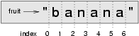
If you imagine this as a piece of paper, the slice operator [n:m] copies out the part of the paper between the n and m positions. Provided m and n are both within the bounds of the string, your result will be of length (m-n).
Three tricks are added to this: if you omit the first index (before the colon), the slice starts at the beginning of the string (or list). If you omit the second index, the slice extends to the end of the string (or list). Similarly, if you provide value for n that is bigger than the length of the string (or list), the slice will take all the values up to the end. (It won't give an "out of range" error like the normal indexing operation does.) Thus:
>>> fruit = "banana" >>> fruit[:3] 'ban' >>> fruit[3:] 'ana' >>> fruit[3:999] 'ana'
What do you think s[:] means? What about friends[4:]?
String comparison
The comparison operators work on strings. To see if two strings are equal:
if word == "banana": print("Yes, we have no bananas!")
Other comparison operations are useful for putting words in lexicographical order:
if word < "banana": print("Your word, " + word + ", comes before banana.") elif word > "banana": print("Your word, " + word + ", comes after banana.") else: print("Yes, we have no bananas!")
This is similar to the alphabetical order you would use with a dictionary, except that all the uppercase letters come before all the lowercase letters. As a result:
Your word, Zebra, comes before banana.
A common way to address this problem is to convert strings to a standard format, such as all lowercase, before performing the comparison. A more difficult problem is making the program realize that zebras are not fruit.
Strings are immutable
It is tempting to use the [] operator on the left side of an assignment, with the intention of changing a character in a string. For example:
greeting = "Hello, world!" greeting[0] = 'J' # ERROR! print(greeting)
Instead of producing the output Jello, world!, this code produces the runtime error TypeError: 'str' object does not support item assignment.
Strings are immutable, which means you can't change an existing string. The best you can do is create a new string that is a variation on the original:
greeting = "Hello, world!" new_greeting = "J" + greeting[1:] print(new_greeting)
The solution here is to concatenate a new first letter onto a slice of greeting. This operation has no effect on the original string.
A find function
What does the following function do?
def find(strng, ch): """ Find and return the index of ch in strng. Return -1 if ch does not occur in strng. """ ix = 0 while ix < len(strng): if strng[ix] == ch: return ix ix += 1 return -1 test(find("Compsci", "p") == 3) test(find("Compsci", "C") == 0) test(find("Compsci", "i") == 6) test(find("Compsci", "x") == -1)
In a sense, find is the opposite of the indexing operator. Instead of taking an index and extracting the corresponding character, it takes a character and finds the index where that character appears. If the character is not found, the function returns -1.
This is another example where we see a return statement inside a loop. If strng[ix] == ch, the function returns immediately, breaking out of the loop prematurely.
If the character doesn't appear in the string, then the program exits the loop normally and returns -1.
This pattern of computation is sometimes called a eureka traversal or short-circuit evaluation, because as soon as we find what we are looking for, we can cry "Eureka!", take the short-circuit, and stop looking.
Looping and counting
The following program counts the number of times the letter a appears in a string, and is another example of the counter pattern introduced in counting:
def count_a(text): count = 0 for c in text: if c == "a": count += 1 return(count) test(count_a("banana") == 3)
Optional parameters (Optional topic)
Python offers powerful features that make programming easier for experienced programmers. One such feature are optional parameters. You are encouraged to read about them; many Python programmers often use optional parameters. However, if you are just starting as a programmer, you are free to skip this section; this topic is not mandatory within this course.
To understand why optional parameters are useful, consider the following example. Suppose we want to find the first occurrence of a character in a string, considering only locations in the string starting from a given location. We can modify the find function, adding a third parameter for the starting position in the search string:
def find2(strng, ch, start): ix = start while ix < len(strng): if strng[ix] == ch: return ix ix += 1 return -1 test(find2("banana", "a", 2) == 3)
The call find2("banana", "a", 2) now returns 3, the index of the first occurrence of "a" in "banana" starting the search at index 2. What does find2("banana", "n", 3) return? If you said 3, there is a good chance you understand how find2 works.
Better still, we can combine find and find2 using an optional parameter:
def find(strng, ch, start=0): ix = start while ix < len(strng): if strng[ix] == ch: return ix ix += 1 return -1
When a function has an optional parameter, the caller may provide a matching argument. If the third argument is provided to find, it gets assigned to start. But if the caller leaves the argument out, then start is given a default value indicated by the assignment start=0 in the function definition.
So the call find("banana", "a", 2) to this version of find behaves just like find2, while in the call find("banana", "a"), start will be set to the default value of 0.
Adding another optional parameter to find makes it search from a starting position, up to but not including the end position:
def find(strng, ch, start=0, end=None): ix = start if end is None: end = len(strng) while ix < end: if strng[ix] == ch: return ix ix += 1 return -1
The optional value for end is interesting: we give it a default value None if the caller does not supply any argument. In the body of the function we test what end is, and if the caller did not supply any argument, we reassign end to be the length of the string. If the caller has supplied an argument for end, however, the caller's value will be used in the loop.
The semantics of start and end in this function are precisely the same as they are in the range function.
Here are some test cases that should pass:
ss = "Python strings have some interesting methods." test(find(ss, "s") == 7) test(find(ss, "s", 7) == 7) test(find(ss, "s", 8) == 13) test(find(ss, "s", 8, 13) == -1) test(find(ss, ".") == len(ss)-1)
The in and not in operators (Optional topic)
The in operator tests for membership. When both of the arguments to in are strings, in checks whether the left argument is a substring of the right argument.
>>> "p" in "apple" True >>> "i" in "apple" False >>> "ap" in "apple" True >>> "pa" in "apple" False
Note that a string is a substring of itself, and the empty string is a substring of any other string. (Also note that computer scientists like to think about these edge cases quite carefully!)
>>> "a" in "a" True >>> "apple" in "apple" True >>> "" in "a" True >>> "" in "apple" True
The not in operator returns the logical opposite results of in:
>>> "x" not in "apple" True
Combining the in operator with string concatenation using +, we can write a function that removes all the vowels from a string:
def remove_vowels(s): vowels = "aeiouAEIOU" s_sans_vowels = "" for x in s: if x not in vowels: s_sans_vowels += x return s_sans_vowels test(remove_vowels("compsci") == "cmpsc") test(remove_vowels("aAbEefIijOopUus") == "bfjps")
The built-in find method (Optional topic)
Now that we've done all this work to write a powerful find function, we can reveal that strings already have their own built-in find method. It can do everything that our code can do, and more!
test(ss.find("s") == 7) test(ss.find("s", 7) == 7) test(ss.find("s", 8) == 13) test(ss.find("s", 8, 13) == -1) test(ss.find(".") == len(ss)-1)
The built-in find method is more general than our version. It can find substrings, not just single characters:
>>> "banana".find("nan") 2 >>> "banana".find("na", 3) 4
Usually we'd prefer to use the methods that Python provides rather than reinvent our own equivalents. But many of the built-in functions and methods make good teaching exercises, and the underlying techniques you learn are your building blocks to becoming a proficient programmer.
The split method (Optional topic)
One of the most useful methods on strings is the split method: it splits a single multi-word string into a list of individual words, removing all the whitespace between them. (Whitespace means any tabs, newlines, or spaces.) This allows us to read input as a single string, and split it into words.
>>> ss = "Well I never did said Alice" >>> wds = ss.split() >>> wds ['Well', 'I', 'never', 'did', 'said', 'Alice']
Cleaning up your strings (Optional topic)
We'll often work with strings that contain punctuation, or tab and newline characters, especially, as we'll see in a future chapter, when we read our text from files or from the Internet. But if we're writing a program, say, to count word frequencies or check the spelling of each word, we'd prefer to strip off these unwanted characters.
We'll show just one example of how to strip punctuation from a string. Remember that strings are immutable, so we cannot change the string with the punctuation --- we need to traverse the original string and create a new string, omitting any punctuation:
punctuation = "!\"#$%&'()*+,-./:;<=>?@[\\]^_`{|}~" def remove_punctuation(s): s_sans_punct = "" for letter in s: if letter not in punctuation: s_sans_punct += letter return s_sans_punct
Setting up that first assignment is messy and error-prone. Fortunately, the Python string module already does it for us. So we will make a slight improvement to this program --- we'll import the string module and use its definition:
import string def remove_punctuation(s): s_without_punct = "" for letter in s: if letter not in string.punctuation: s_without_punct += letter return s_without_punct test(remove_punctuation('"Well, I never did!", said Alice.') == "Well I never did said Alice") test(remove_punctuation("Are you very, very, sure?") == "Are you very very sure")
Composing together this function and the split method from the previous section makes a useful combination --- we'll clean out the punctuation, and split will clean out the newlines and tabs while turning the string into a list of words:
my_story = """ Pythons are constrictors, which means that they will 'squeeze' the life out of their prey. They coil themselves around their prey and with each breath the creature takes the snake will squeeze a little tighter until they stop breathing completely. Once the heart stops the prey is swallowed whole. The entire animal is digested in the snake's stomach except for fur or feathers. What do you think happens to the fur, feathers, beaks, and eggshells? The 'extra stuff' gets passed out as --- you guessed it --- snake POOP! """ wds = remove_punctuation(my_story).split() print(wds)
The output:
['Pythons', 'are', 'constrictors', ... , 'it', 'snake', 'POOP']
As indicated earlier, there are other useful string methods, but this book isn't intended to be a reference manual. You can find all necessary information in the Python Library Reference online.
The string format method (Optional topic)
The easiest and most powerful way to format a string in Python 3 is to use the format method. To see how this works, let's start with a few examples:
s1 = "His name is {0}!".format("Arthur") print(s1) name = "Alice" age = 10 s2 = "I am {1} and I am {0} years old.".format(age, name) print(s2) n1 = 4 n2 = 5 s3 = "2**10 = {0} and {1} * {2} = {3:f}".format(2**10, n1, n2, n1 * n2) print(s3)
Running the script produces:
His name is Arthur! I am Alice and I am 10 years old. 2**10 = 1024 and 4 * 5 = 20.000000
The template string contains place holders, ... {0} ... {1} ... {2} ... etc. The format method substitutes its arguments into the place holders. The numbers in the place holders are indexes that determine which argument gets substituted --- make sure you understand line 6 above!
But there's more! Each of the replacement fields can also contain a format specification --- it is always introduced by the : symbol (Line 11 above uses one.) This modifies how the substitutions are made into the template, and can control things like:
- whether the field is aligned to the left <, center ^, or right >
- the width allocated to the field within the result string (a number like 10)
- the type of conversion (we'll initially only force conversion to float, f, as we did in line 11 of the code above, or perhaps we'll ask integer numbers to be converted to hexadecimal using x)
- if the type conversion is a float, you can also specify how many decimal places are wanted (typically, .2f is useful for working with currencies to two decimal places.)
Let's do a few simple and common examples that should be enough for most needs. If you need to do anything more esoteric, use help and read all the powerful, gory details.
n1 = "Paris" n2 = "Whitney" n3 = "Hilton" print("Pi to three decimal places is {0:.3f}".format(3.1415926)) print("123456789 123456789 123456789 123456789 123456789 123456789") print("|||{0:<15}|||{1:^15}|||{2:>15}|||Born in {3}|||" .format(n1,n2,n3,1981)) print("The decimal value {0} converts to hex value {0:x}" .format(123456))
This script produces the output:
Pi to three decimal places is 3.142 123456789 123456789 123456789 123456789 123456789 123456789 |||Paris ||| Whitney ||| Hilton|||Born in 1981||| The decimal value 123456 converts to hex value 1e240
You can have multiple placeholders indexing the same argument, or perhaps even have extra arguments that are not referenced at all:
letter = """ Dear {0} {2}. {0}, I have an interesting money-making proposition for you! If you deposit $10 million into my bank account, I can double your money ... """ print(letter.format("Paris", "Whitney", "Hilton")) print(letter.format("Bill", "Henry", "Gates"))
This produces the following:
Dear Paris Hilton. Paris, I have an interesting money-making proposition for you! If you deposit $10 million into my bank account, I can double your money ... Dear Bill Gates. Bill, I have an interesting money-making proposition for you! If you deposit $10 million into my bank account I can double your money ...
As you might expect, you'll get an index error if your placeholders refer to arguments that you do not provide:
>>> "hello {3}".format("Dave") Traceback (most recent call last): File "<interactive input>", line 1, in <module> IndexError: tuple index out of range
The following example illustrates the real utility of string formatting. First, we'll try to print a table without using string formatting:
print("i\ti**2\ti**3\ti**5\ti**10\ti**20") for i in range(1, 11): print(i, "\t", i**2, "\t", i**3, "\t", i**5, "\t", i**10, "\t", i**20)
This program prints out a table of various powers of the numbers from 1 to 10. (This assumes that the tab width is 8. You might see something even worse than this if you tab width is set to 4.) In its current form it relies on the tab character ( \t) to align the columns of values, but this breaks down when the values in the table get larger than the tab width:
i i**2 i**3 i**5 i**10 i**20 1 1 1 1 1 1 2 4 8 32 1024 1048576 3 9 27 243 59049 3486784401 4 16 64 1024 1048576 1099511627776 5 25 125 3125 9765625 95367431640625 6 36 216 7776 60466176 3656158440062976 7 49 343 16807 282475249 79792266297612001 8 64 512 32768 1073741824 1152921504606846976 9 81 729 59049 3486784401 12157665459056928801 10 100 1000 100000 10000000000 100000000000000000000
One possible solution would be to change the tab width, but the first column already has more space than it needs. The best solution would be to set the width of each column independently. As you may have guessed by now, string formatting provides a much nicer solution. We can also right-justify each field:
layout = "{0:>4}{1:>6}{2:>6}{3:>8}{4:>13}{5:>24}" print(layout.format("i", "i**2", "i**3", "i**5", "i**10", "i**20")) for i in range(1, 11): print(layout.format(i, i**2, i**3, i**5, i**10, i**20))
Running this version produces the following (much more satisfying) output:
i i**2 i**3 i**5 i**10 i**20 1 1 1 1 1 1 2 4 8 32 1024 1048576 3 9 27 243 59049 3486784401 4 16 64 1024 1048576 1099511627776 5 25 125 3125 9765625 95367431640625 6 36 216 7776 60466176 3656158440062976 7 49 343 16807 282475249 79792266297612001 8 64 512 32768 1073741824 1152921504606846976 9 81 729 59049 3486784401 12157665459056928801 10 100 1000 100000 10000000000 100000000000000000000
Summary
This chapter introduced a lot of new ideas. The following summary may prove helpful in remembering what you learned.
- indexing ([])
- Access a single character in a string using its position (starting from 0). Example: "This"[2] evaluates to "i".
- length function (len)
- Returns the number of characters in a string. Example: len("happy") evaluates to 5.
- for loop traversal (for)
Traversing a string means accessing each character in the string, one at a time. For example, the following for loop:
for ch in "Example": ...executes the body of the loop 7 times with different values of ch each time.
- slicing ([:])
- A slice is a substring of a string. Example: 'bananas and cream'[3:6] evaluates to ana (so does 'bananas and cream'[1:4]).
- string comparison (>, <, >=, <=, ==, !=)
- The six common comparison operators work with strings, evaluating according to lexicographical order. Examples: "apple" < "banana" evaluates to True. "Zeta" < "Appricot" evaluates to False. "Zebra" <= "aardvark" evaluates to True because all upper case letters precede lower case letters.
- in and not in operator (in, not in)
- The in operator tests for membership. In the case of strings, it tests whether one string is contained inside another string. Examples: "heck" in "I'll be checking for you." evaluates to True. "cheese" in "I'll be checking for you." evaluates to False.
Glossary
- compound data type
- A data type in which the values are made up of components, or elements, that are themselves values.
- default value
- The value given to an optional parameter if no argument for it is provided in the function call.
- docstring
- A string constant on the first line of a function or module definition (and as we will see later, in class and method definitions as well). Docstrings provide a convenient way to associate documentation with code. Docstrings are also used by programming tools to provide interactive help.
- dot notation
- Use of the dot operator, ., to access methods and attributes of an object.
- immutable data value
- A data value which cannot be modified. Assignments to elements or slices (sub-parts) of immutable values cause a runtime error.
- index
- A variable or value used to select a member of an ordered collection, such as a character from a string, or an element from a list.
- mutable data value
- A data value which can be modified. The types of all mutable values are compound types. Lists and dictionaries are mutable; strings and tuples are not.
- optional parameter
- A parameter written in a function header with an assignment to a default value which it will receive if no corresponding argument is given for it in the function call.
- short-circuit evaluation
- A style of programming that shortcuts extra work as soon as the outcome is know with certainty. In this chapter our find function returned as soon as it found what it was looking for; it didn't traverse all the rest of the items in the string.
- slice
- A part of a string (substring) specified by a range of indices. More generally, a subsequence of any sequence type in Python can be created using the slice operator (sequence[start:stop]).
- traverse
- To iterate through the elements of a collection, performing a similar operation on each.
- whitespace
- Any of the characters that move the cursor without printing visible characters. The constant string.whitespace contains all the white-space characters.
References
| [ThinkCS] | How To Think Like a Computer Scientist --- Learning with Python 3 |
Lists
Source: this section is heavily based on Chapter 11 of [ThinkCS].
A list is an ordered collection of values. The values that make up a list are called its elements, or its items. We will use the term element or item to mean the same thing. Lists are similar to strings, which are ordered collections of characters, except that the elements of a list can be of any type. Lists and strings --- and other collections that maintain the order of their items --- are called sequences.
List values
There are several ways to create a new list; the simplest is to enclose the elements in square brackets ([ and ]):
ps = [10, 20, 30, 40] qs = ["spam", "bungee", "swallow"]
The first example is a list of four integers. The second is a list of three strings. The elements of a list don't have to be the same type. The following list contains a string, a float, an integer, and (amazingly) another list:
zs = ["hello", 2.0, 5, [10, 20]]
A list within another list is said to be nested.
Finally, a list with no elements is called an empty list, and is denoted [].
We have already seen that we can assign list values to variables or pass lists as parameters to functions:
>>> vocabulary = ["apple", "cheese", "dog"] >>> numbers = [17, 123] >>> an_empty_list = [] >>> print(vocabulary, numbers, an_empty_list) ["apple", "cheese", "dog"] [17, 123] []
Accessing elements
The syntax for accessing the elements of a list is the same as the syntax for accessing the characters of a string --- the index operator: [] (not to be confused with an empty list). The expression inside the brackets specifies the index. Remember that the indices start at 0:
>>> numbers[0] 17
Any expression evaluating to an integer can be used as an index:
>>> numbers[9-8] 5 >>> numbers[1.0] Traceback (most recent call last): File "<interactive input>", line 1, in <module> TypeError: list indices must be integers, not float
If you try to access or assign to an element that does not exist, you get a runtime error:
>>> numbers[2] Traceback (most recent call last): File "<interactive input>", line 1, in <module> IndexError: list index out of range
It is common to use a loop variable as a list index.
horsemen = ["war", "famine", "pestilence", "death"] for i in [0, 1, 2, 3]: print(horsemen[i])
Each time through the loop, the variable i is used as an index into the list, printing the i'th element. This pattern of computation is called a list traversal.
The above sample doesn't need or use the index i for anything besides getting the items from the list, so this more direct version --- where the for loop gets the items --- might be preferred:
horsemen = ["war", "famine", "pestilence", "death"] for h in horsemen: print(h)
List length
The function len returns the length of a list, which is equal to the number of its elements. If you are going to use an integer index to access the list, it is a good idea to use this value as the upper bound of a loop instead of a constant. That way, if the size of the list changes, you won't have to go through the program changing all the loops; they will work correctly for any size list:
horsemen = ["war", "famine", "pestilence", "death"] for i in range(len(horsemen)): print(horsemen[i])
The last time the body of the loop is executed, i is len(horsemen) - 1, which is the index of the last element. (But the version without the index looks even better now!)
Although a list can contain another list, the nested list still counts as a single element in its parent list. The length of this list is 4:
>>> len(["car makers", 1, ["Ford", "Toyota", "BMW"], [1, 2, 3]]) 4
List membership (Optional topic)
in and not in are Boolean operators that test membership in a sequence. We used them previously with strings, but they also work with lists and other sequences:
>>> horsemen = ["war", "famine", "pestilence", "death"] >>> "pestilence" in horsemen True >>> "debauchery" in horsemen False >>> "debauchery" not in horsemen True
Using this produces a more elegant version of the nested loop program we previously used to count the number of students doing Computer Science in the section nested_data:
students = [ ("John", ["CompSci", "Physics"]), ("Vusi", ["Maths", "CompSci", "Stats"]), ("Jess", ["CompSci", "Accounting", "Economics", "Management"]), ("Sarah", ["InfSys", "Accounting", "Economics", "CommLaw"]), ("Zuki", ["Sociology", "Economics", "Law", "Stats", "Music"])] # Count how many students are taking CompSci counter = 0 for (name, subjects) in students: if "CompSci" in subjects: counter += 1 print("The number of students taking CompSci is", counter)
List operations
The + operator concatenates lists:
>>> a = [1, 2, 3] >>> b = [4, 5, 6] >>> c = a + b >>> c [1, 2, 3, 4, 5, 6]
Similarly, the * operator repeats a list a given number of times:
>>> [0] * 4 [0, 0, 0, 0] >>> [1, 2, 3] * 3 [1, 2, 3, 1, 2, 3, 1, 2, 3]
The first example repeats [0] four times. The second example repeats the list [1, 2, 3] three times.
List slices
The slice operations we saw previously with strings let us work with sublists:
>>> a_list = ["a", "b", "c", "d", "e", "f"] >>> a_list[1:3] ['b', 'c'] >>> a_list[:4] ['a', 'b', 'c', 'd'] >>> a_list[3:] ['d', 'e', 'f'] >>> a_list[:] ['a', 'b', 'c', 'd', 'e', 'f']
Lists are mutable
Unlike strings, lists are mutable, which means we can change their elements. Using the index operator on the left side of an assignment, we can update one of the elements:
>>> fruit = ["banana", "apple", "quince"] >>> fruit[0] = "pear" >>> fruit[2] = "orange" >>> fruit ['pear', 'apple', 'orange']
The bracket operator applied to a list can appear anywhere in an expression. When it appears on the left side of an assignment, it changes one of the elements in the list, so the first element of fruit has been changed from "banana" to "pear", and the last from "quince" to "orange". An assignment to an element of a list is called item assignment. Item assignment does not work for strings:
>>> my_string = "TEST" >>> my_string[2] = "X" Traceback (most recent call last): File "<interactive input>", line 1, in <module> TypeError: 'str' object does not support item assignment
but it does for lists:
>>> my_list = ["T", "E", "S", "T"] >>> my_list[2] = "X" >>> my_list ['T', 'E', 'X', 'T']
With the slice operator we can update a whole sublist at once:
>>> a_list = ["a", "b", "c", "d", "e", "f"] >>> a_list[1:3] = ["x", "y"] >>> a_list ['a', 'x', 'y', 'd', 'e', 'f']
We can also remove elements from a list by assigning an empty list to them:
>>> a_list = ["a", "b", "c", "d", "e", "f"] >>> a_list[1:3] = [] >>> a_list ['a', 'd', 'e', 'f']
And we can add elements to a list by squeezing them into an empty slice at the desired location:
>>> a_list = ["a", "d", "f"] >>> a_list[1:1] = ["b", "c"] >>> a_list ['a', 'b', 'c', 'd', 'f'] >>> a_list[4:4] = ["e"] >>> a_list ['a', 'b', 'c', 'd', 'e', 'f']
List deletion
Using slices to delete list elements can be error-prone. Python provides an alternative that is more readable. The del statement removes an element from a list:
>>> a = ["one", "two", "three"] >>> del a[1] >>> a ['one', 'three']
As you might expect, del causes a runtime error if the index is out of range.
You can also use del with a slice to delete a sublist:
>>> a_list = ["a", "b", "c", "d", "e", "f"] >>> del a_list[1:5] >>> a_list ['a', 'f']
As usual, the sublist selected by slice contains all the elements up to, but not including, the second index.
Objects and references
After we execute these assignment statements
a = "banana" b = "banana"
we know that a and b will refer to a string object with the letters "banana". But we don't know yet whether they point to the same string object.
There are two possible ways the Python interpreter could arrange its memory:
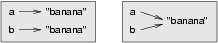
In one case, a and b refer to two different objects that have the same value. In the second case, they refer to the same object.
We can test whether two names refer to the same object using the is operator:
>>> a is b True
This tells us that both a and b refer to the same object, and that it is the second of the two state snapshots that accurately describes the relationship.
Since strings are immutable, Python optimizes resources by making two names that refer to the same string value refer to the same object.
This is not the case with lists:
>>> a = [1, 2, 3] >>> b = [1, 2, 3] >>> a == b True >>> a is b False
The state snapshot here looks like this:
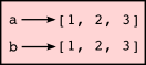
a and b will then have the same value but do not refer to the same object.
Aliasing
Since variables refer to objects, if we assign one variable to another, both variables refer to the same object:
>>> a = [1, 2, 3] >>> b = a >>> a is b True
In this case, the state snapshot looks like this:
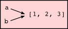
Because the same list has two different names, a and b, we say that it is aliased. Changes made with one alias affect the other:
>>> b[0] = 5 >>> a [5, 2, 3]
Although this behavior can be useful, it is sometimes unexpected or undesirable. In general, it is safer to avoid aliasing when you are working with mutable objects (i.e. lists at this point in our textbook, but we'll meet more mutable objects as we cover classes and objects, dictionaries and sets). Of course, for immutable objects (i.e. strings), there's no problem --- it is just not possible to change something and get a surprise when you access an alias name. That's why Python is free to alias strings (and any other immutable kinds of data) when it sees an opportunity to economize.
Cloning lists
If we want to modify a list and also keep a copy of the original, we need to be able to make a copy of the list itself, not just the reference. This process is sometimes called cloning, to avoid the ambiguity of the word copy.
The easiest way to clone a list is to use the slice operator:
>>> a = [1, 2, 3] >>> b = a[:] >>> b [1, 2, 3]
Taking any slice of a creates a new list. In this case the slice happens to consist of the whole list. So now the relationship is like this:
Now we are free to make changes to b without worrying that we'll inadvertently be changing a:
>>> b[0] = 5 >>> a [1, 2, 3]
Lists and for loops
The for loop also works with lists, as we've already seen. The generalized syntax of a for loop is:
for VARIABLE in LIST: BODY
So, as we've seen
friends = ["Joe", "Zoe", "Brad", "Angelina", "Zuki", "Thandi", "Paris"] for friend in friends: print(friend)
It almost reads like English: For (every) friend in (the list of) friends, print (the name of the) friend.
Any list expression can be used in a for loop:
for number in range(20): if number % 3 == 0: print(number) for fruit in ["banana", "apple", "quince"]: print("I like to eat " + fruit + "s!")
The first example prints all the multiples of 3 between 0 and 19. The second example expresses enthusiasm for various fruits.
Since lists are mutable, we often want to traverse a list, changing each of its elements. The following squares all the numbers in the list xs:
xs = [1, 2, 3, 4, 5] for i in range(len(xs)): xs[i] = xs[i]**2
Take a moment to think about range(len(xs)) until you understand how it works.
List parameters
Passing a list as an argument actually passes a reference to the list, not a copy or clone of the list. So parameter passing creates an alias for you: the caller has one variable referencing the list, and the called function has an alias, but there is only one underlying list object. For example, the function below takes a list as an argument and multiplies each element in the list by 2:
def double_stuff(a_list): """ Overwrite each element in a_list with double its value. """ for i in range(len(a_list)): a_list[i] = 2 * a_list[i]
If we add the following onto our script:
things = [2, 5, 9] double_stuff(things) print(things)
When we run it we'll get:
[4, 10, 18]
In the function above, the parameter a_list and the variable things are aliases for the same object. So before any changes to the elements in the list, the state snapshot looks like this:
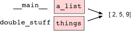
Since the list object is shared by two frames, we drew it between them.
If a function modifies the items of a list parameter, the caller sees the change.
Use the Python visualizer!
We've already mentioned the Python visualizer at http://www.pythontutor.com/visualize.html. It is a very useful tool for building a good understanding of references, aliases, assignments, and passing arguments to functions. Pay special attention to cases where you clone a list or have two separate lists, and cases where there is only one underlying list, but more than one variable is aliased to reference the list.
List methods
The dot operator can also be used to access built-in methods of list objects. We'll start with the most useful method for adding something onto the end of an existing list:
>>> mylist = [] >>> mylist.append(5) >>> mylist.append(27) >>> mylist.append(3) >>> mylist.append(12) >>> mylist [5, 27, 3, 12]
append is a list method which adds the argument passed to it to the end of the list. We'll use it heavily when we're creating new lists. Continuing with this example, we show several other list methods:
>>> mylist.insert(1, 12) # Insert 12 at pos 1, shift other items up >>> mylist [5, 12, 27, 3, 12] >>> mylist.count(12) # How many times is 12 in mylist? 2 >>> mylist.extend([5, 9, 5, 11]) # Put whole list onto end of mylist >>> mylist [5, 12, 27, 3, 12, 5, 9, 5, 11]) >>> mylist.index(9) # Find index of first 9 in mylist 6 >>> mylist.reverse() >>> mylist [11, 5, 9, 5, 12, 3, 27, 12, 5] >>> mylist.sort() >>> mylist [3, 5, 5, 5, 9, 11, 12, 12, 27] >>> mylist.remove(12) # Remove the first 12 in the list >>> mylist [3, 5, 5, 5, 9, 11, 12, 27]
Experiment and play with the list methods shown here, and read their documentation until you feel confident that you understand how they work. You are not required to learn these functions by heart and are always free to check Python's documentation to understand what these functions are doing.
Python also provides built-in functions that can be applied to lists. One example is the sorted function.
>>> mylist = [5, 27, 3, 12] >>> sorted ( mylist ) [3, 5, 1, 27] >>> mylist [5, 27, 3, 12]
The difference between sorted and sort is that sorted returns a sorted version of the list, and keeps the original list unmodified.
Pure functions and modifiers
Functions which take lists as arguments and change them during execution are called modifiers and the changes they make are called side effects.
A pure function does not produce side effects. It communicates with the calling program only through parameters, which it does not modify, and a return value. Here is double_stuff written as a pure function:
def double_stuff(a_list): """ Return a new list which contains doubles of the elements in a_list. """ new_list = [] for value in a_list: new_elem = 2 * value new_list.append(new_elem) return new_list
This version of double_stuff does not change its arguments:
>>> things = [2, 5, 9] >>> xs = double_stuff(things) >>> things [2, 5, 9] >>> xs [4, 10, 18]
An early rule we saw for assignment said "first evaluate the right hand side, then assign the resulting value to the variable". So it is quite safe to assign the function result to the same variable that was passed to the function:
>>> things = [2, 5, 9] >>> things = double_stuff(things) >>> things [4, 10, 18]
Which style is better?
Anything that can be done with modifiers can also be done with pure functions. In fact, some programming languages only allow pure functions. There is some evidence that programs that use pure functions are faster to develop and less error-prone than programs that use modifiers. Nevertheless, modifiers are convenient at times, and in some cases, functional programs are less efficient.
In general, we recommend that you write pure functions whenever it is reasonable to do so and resort to modifiers only if there is a compelling advantage. This approach might be called a functional programming style.
Functions that produce lists
The pure version of double_stuff above made use of an important pattern for your toolbox. Whenever you need to write a function that creates and returns a list, the pattern is usually:
initialize a result variable to be an empty list loop create a new element append it to result return the result
Let us show another use of this pattern. Assume you already have a function is_prime(x) that can test if x is prime. Write a function to return a list of all prime numbers less than n:
def primes_lessthan(n): """ Return a list of all prime numbers less than n. """ result = [] for i in range(2, n): if is_prime(i): result.append(i) return result
Strings and lists (Optional topic)
Two useful methods on strings involve conversion to and from lists of substrings. We will see these in more detail when discussing how to read files; however, feel free to read a little about them at this moment already. The split method breaks a string into a list of words. By default, any number of whitespace characters is considered a word boundary:
>>> song = "The rain in Spain..." >>> wds = song.split() >>> wds ['The', 'rain', 'in', 'Spain...']
An optional argument called a delimiter can be used to specify which string to use as the boundary marker between substrings. The following example uses the string ai as the delimiter:
>>> song.split("ai") ['The r', 'n in Sp', 'n...']
Notice that the delimiter doesn't appear in the result.
The inverse of the split method is join. You choose a desired separator string, (often called the glue) and join the list with the glue between each of the elements:
>>> glue = ";" >>> s = glue.join(wds) >>> s 'The;rain;in;Spain...'
The list that you glue together (wds in this example) is not modified. Also, as these next examples show, you can use empty glue or multi-character strings as glue:
>>> " --- ".join(wds) 'The --- rain --- in --- Spain...' >>> "".join(wds) 'TheraininSpain...'
list and range
Python has a built-in type conversion function called list that tries to turn whatever you give it into a list.
>>> xs = list("Crunchy Frog") >>> xs ["C", "r", "u", "n", "c", "h", "y", " ", "F", "r", "o", "g"] >>> "".join(xs) 'Crunchy Frog'
One particular feature of range is that it doesn't instantly compute all its values: it "puts off" the computation, and does it on demand, or "lazily". We'll say that it gives a promise to produce the values when they are needed. This is very convenient if your computation short-circuits a search and returns early, as in this case:
def f(n): """ Find the first positive integer between 101 and less than n that is divisible by 21 """ for i in range(101, n): if (i % 21 == 0): return i test(f(110) == 105) test(f(1000000000) == 105)
In the second test, if range were to eagerly go about building a list with all those elements, you would soon exhaust your computer's available memory and crash the program. But it is cleverer than that! This computation works just fine, because the range object is just a promise to produce the elements if and when they are needed. Once the condition in the if becomes true, no further elements are generated, and the function returns. (Note: Before Python 3, range was not lazy. If you use an earlier versions of Python, YMMV!)
YMMV: Your Mileage May Vary
The acronym YMMV stands for your mileage may vary. American car advertisements often quoted fuel consumption figures for cars, e.g. that they would get 28 miles per gallon. But this always had to be accompanied by legal small-print warning the reader that they might not get the same. The term YMMV is now used idiomatically to mean "your results may differ", e.g. The battery life on this phone is 3 days, but YMMV.
You'll sometimes find the lazy range wrapped in a call to list. This forces Python to turn the lazy promise into an actual list:
>>> range(10) # Create a lazy promise range(0, 10) >>> list(range(10)) # Call in the promise, to produce a list. [0, 1, 2, 3, 4, 5, 6, 7, 8, 9]
List Comprehension (Optional topic)
Let us reconsider the double_stuff function:
def double_stuff(a_list): """ Return a new list which contains doubles of the elements in a_list. """ new_list = [] for value in a_list: new_elem = 2 * value new_list.append(new_elem) return new_list
While this function is correct, the developers of Python felt that this notation is longer than desirable: in Python one often wishes to create lists based on other lists. For this reason, a shorter notation was introduced in the language. Any program written using this shorter notation, can also be written without it; however, programs much shorter when you use it:
def double_stuff(a_list): """ Return a new list which contains doubles of the elements in a_list. """ return [ 2 * value for value in a_list ]
This notation is known as list comprehension, and is inspired by set-builder notation in mathematics. An equivalent way of writing in mathematics is the following:
In mathematics we can also write statements such as this:
Also this can be transformed directly into Python!
def double_stuff(a_list): """ Return a new list which contains doubles of the elements in a_list that are not lower than 3 """ return [ 2 * value for value in a_list if a>= 3 ]
We can use multiple nested loops in list comprehension as well:
[ x * y for x in [0,1,2] for y in [0,2,4] if x * y >= 3 ]
In mathematics, we would write this as follows:
List comprehension is useful in many contexts. One interesting example in which we can use list comprehension is in the conversion of lists. Suppose we have this list of numbers:
numbers = [1, 3, 5]
and we wish to turn this list into the following strings:
["1", "3", "5"]
Unfortunately, we cannot obtain this string by simply writing str(numbers). The result of str(numbers) is a single string that represents the list of numbers.
To convert every element in a list separately, we can however write:
[ str(number) for number in numbers ]
Here, we apply the str function on every number in the numbers list, and put the result of this function call in the new list.
Glossary
- aliases
- Multiple variables that contain references to the same object.
- clone
- To create a new object that has the same value as an existing object. Copying a reference to an object creates an alias but doesn't clone the object.
- delimiter
- A character or string used to indicate where a string should be split.
- element
- One of the values in a list (or other sequence). The bracket operator selects elements of a list. Also called item.
- immutable data value
- A data value which cannot be modified. Assignments to elements or slices (sub-parts) of immutable values cause a runtime error.
- index
- An integer value that indicates the position of an item in a list. Indexes start from 0.
- item
- See element.
- list
- A collection of values, each in a fixed position within the list. Like other types str, int, float, etc. there is also a list type-converter function that tries to turn whatever argument you give it into a list.
- list traversal
- The sequential accessing of each element in a list.
- modifier
- A function which changes its arguments inside the function body. Only mutable types can be changed by modifiers.
- mutable data value
- A data value which can be modified. The types of all mutable values are compound types. Lists and dictionaries are mutable; strings and tuples are not.
- nested list
- A list that is an element of another list.
- object
- A thing to which a variable can refer.
- pattern
- A sequence of statements, or a style of coding something that has general applicability in a number of different situations. Part of becoming a mature Computer Scientist is to learn and establish the patterns and algorithms that form your toolkit. Patterns often correspond to your "mental chunking".
- promise
- An object that promises to do some work or deliver some values if they're eventually needed, but it lazily puts off doing the work immediately. Calling range produces a promise.
- pure function
- A function which has no side effects. Pure functions only make changes to the calling program through their return values.
- sequence
- Any of the data types that consist of an ordered collection of elements, with each element identified by an index.
- side effect
- A change in the state of a program made by calling a function. Side effects can only be produced by modifiers.
- step size
- The interval between successive elements of a linear sequence. The third (and optional argument) to the range function is called the step size. If not specified, it defaults to 1.
References
| [ThinkCS] | How To Think Like a Computer Scientist --- Learning with Python 3 |
Nested Datastructures
Source: this section combines elements of Chapters 7 and 11 of [ThinkCS].
In the previous sections, we introduced strings and lists as individual data structures. In practice, these data structures are often used in combination with each other. We will show a number of such cases in this section.
Nested lists
A nested list is a list that appears as an element in another list. In this list, the element with index 3 is a nested list:
>>> nested = ["hello", 2.0, 5, [10, 20]]
If we output the element at index 3, we get:
>>> print(nested[3]) [10, 20]
To extract an element from the nested list, we can proceed in two steps:
>>> elem = nested[3] >>> elem[0] 10
Or we can combine them:
>>> nested[3][1] 20
Bracket operators evaluate from left to right, so this expression gets the 3'th element of nested and extracts the 1'th element from it.
Matrices
Nested lists are often used to represent matrices. For example, consider this matrix:
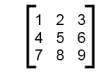 >>> mx = [[1, 2, 3], [4, 5, 6], [7, 8, 9]]
mx is a list with three elements, where each element is a row of the matrix. We can select an entire row from the matrix in the usual way:
>>> mx[1] [4, 5, 6]
Or we can extract a single element from the matrix using the double-index form:
>>> mx[1][2] 6
The first index selects the row, and the second index selects the column. Although this way of representing matrices is common, it is not the only possibility. A small variation is to use a list of columns instead of a list of rows. Later we will see a more radical alternative using a dictionary.
An interesting question is how we can create a matrix of arbitrary size in a practical manner. Many solutions are possible, some of which are more readable than others. This is full code that creates a matrix using the append method:
def matrix(n): """ Returns an n times n matrix with zeros, represented using lists within lists """ m = [] for j in range(n): l = [] for i in range(n): l.append ( 0 ) m.append ( l ) return m
In this code, m is the matrix we are going to return. Within this list, we are creating n nested lists. Each of these nested lists is a list of n 0s.
It could be tempting to write this code instead:
def matrix_incorrect(n): l = [] for i in range(n): l.append ( 0 ) m = [] for j in range(n): m.append ( l ) return m
At first sight, it may seem that this code is correct. If you execute print(matrix_incorrect(3)) you will indeed see this output:
[[0, 0, 0], [0, 0, 0], [0, 0, 0]]
However, the data structure created by this function has undesirable properties. If we execute the following code:
m = matrix_incorrect(3) m[0][0] = 1 print(m)
we will see the following output:
[[1, 0, 0], [1, 0, 0], [1, 0, 0]]
This is most likely not the output that you were looking for; indeed, any modification of one row, will also lead to a modification of the other rows.
The explanation for this can be found in how Python deals with objects and references. The append method takes as argument a reference to an object, and will add a reference to this object to the list. In our code, we have first created a list for which l is a reference. Subsequently, we add this reference three times to the list m. As a result, all three elements in the list m point towards the same underlying list. As m[0], m[1], m[2] all point towards the same list, any change to m[0] will also be visible when printing m[1] and m[2].
Our original code did not have this problem, as we created a new nested list n times.
The following code would avoid this problem:
def matrix_incorrect(n): l = [] for i in range(n): l.append ( 0 ) m = [] for j in range(n): m.append ( list(l) ) return m
The main difference is here that we use the list(l) construction. This construction will first create a copy of l: it will create a new list object that contains the same elements as l; the reference to this new object is added t the list m. As we create n copies of the original list l, all these nested lists are now independent of each other.
Glossary
- nested list
- A list that is an element of another list.
References
| [ThinkCS] | How To Think Like a Computer Scientist --- Learning with Python 3 |
Tuples
Source: this section is heavily based on Chapter 9 of [ThinkCS].
Tuples are used for grouping data
We saw earlier that we could group together pairs of values by surrounding with parentheses. Recall this example:
>>> year_born = ("Paris Hilton", 1981)
The pair is an example of a tuple. This is an example of a data structure --- a mechanism for grouping and organizing data to make it easier to use. Generalizing this, a tuple can be used to group any number of items into a single compound value. Syntactically, a tuple is a comma-separated sequence of values. Although it is not necessary, it is conventional to enclose tuples in parentheses:
>>> julia = ("Julia", "Roberts", 1967, "Duplicity", 2009, "Actress", "Atlanta, Georgia")
Tuples are useful for representing what other languages often call records --- some related information that belongs together, like your student record. There is no description of what each of these fields means, but we can guess. A tuple lets us "chunk" together related information and use it as a single thing.
Tuples are very similar to lists and support the same sequence operations as lists. The index operator selects an element from a tuple:
>>> julia[2] 1967
However, tuples are not the same as lists. Next to the different syntax (parentheses instead of square brackets), an important difference is that tuples are unmutable. If we try to use item assignment to modify one of the elements of the tuple, we get an error:
>>> julia[0] = "X" TypeError: 'tuple' object does not support item assignment
Similarly, we can not add elemnts to a tuple, or remove them; once Python has created a tuple in memory, it cannot be changed.
Of course, even if we can't modify the elements of a tuple, we can always make the julia variable reference a new tuple holding different information. To construct the new tuple, it is convenient that we can slice parts of the old tuple and join up the bits to make the new tuple. So if julia has a new recent film, we could change her variable to reference a new tuple that used some information from the old one:
>>> julia = julia[:3] + ("Eat Pray Love", 2010) + julia[5:] >>> julia ("Julia", "Roberts", 1967, "Eat Pray Love", 2010, "Actress", "Atlanta, Georgia")
To create a tuple with a single element (but you're probably not likely to do that too often), we have to include the final comma, because without the final comma, Python treats the (5) below as an integer in parentheses:
>>> tup = (5,) >>> type(tup) <class 'tuple'> >>> x = (5) >>> type(x) <class 'int'>
Given the similarity between Python's tuples and lists, a good question is why tuples exist at all. Why doesn't Python only have lists? There are two good reasons for the existence of tuples.
One is the performance of the code. Tuples are more efficient than lists: they consume less memory and the run time required to create them is smaller.
Why is this? We skimmed over this till now, but allocating memory in a computer is not a trivial operation; essentially, each time a program requires more memory, the operating system will have to search for a piece of memory that is still unused. This also applies to lists. If the operating system would have to look for a new piece memory each time an element is added to a list, adding elements to a list would be a rather slow operation. To avoid this, Python tries to be intelligent: it will anticipate the addition of elements in a list by reserving more memory than necessary at the moment of creation. The benefit is that adding elements is now faster. The side effect is however that lists will consume more memory than necessary. Python's tuples avoid this. As a tuple will never change, we know its memory consumption will never change. Hence, Python does not need to anticipate future additions to the tuple.
The second reason for having tuples relates to the readability of code written using tuples. Consider this piece of code:
julia = ("Julia", "Roberts", 1967, "Duplicity", 2009, "Actress", "Atlanta, Georgia") do_something ( julia ) print ( julia[0] )
For this piece of code, we can be sure that whatever the functionality of the function do_something is, at the end the string "Julia" will be printed. This makes it easy to understand what the third line of code is doing.
Consider now this piece of code:
julia = ["Julia", "Roberts", 1967, "Duplicity", 2009, "Actress", "Atlanta, Georgia"] do_something ( julia ) print ( julia[0] )
In this code, we can no longer be sure about what julia[0] will print. Consider this implementation of the do_something function:
def do_something ( l ): l[0] = "Hugh"
This function will change the list julia, and as a result the code will print "Hugh". Hence, to understand what the line print ( julia[0] ) does, we will need to check the documentation or source code of the function do_something. For tuples, this is not necessary: by using tuples, the programmer can communicate to another reader of the code that this data is not supposed to be changed. Indeed, any function that you will apply on this tuple, and that would try to change it, will yield an error message, hence making it easier to debug the code as well.
Tuple assignments
Python has a very powerful tuple assignment feature that allows a tuple of variables on the left of an assignment to be assigned values from a tuple on the right of the assignment. (We already saw this used for pairs, but it generalizes.)
(name, surname, b_year, movie, m_year, profession, b_place) = julia
This can also be shortened to
name, surname, b_year, movie, m_year, profession, b_place = julia
This does the equivalent of seven assignment statements, all on one easy line. One requirement is that the number of variables on the left must match the number of elements in the tuple.
One way to think of tuple assignment is as tuple packing/unpacking.
In tuple packing, the values on the left are 'packed' together in a tuple:
>>> b = ("Bob", 19, "CS") # tuple packing
In tuple unpacking, the values in a tuple on the right are 'unpacked' into the variables/names on the right:
>>> b = ("Bob", 19, "CS") >>> (name, age, studies) = b # tuple unpacking >>> name 'Bob' >>> age 19 >>> studies 'CS'
Once in a while, it is useful to swap the values of two variables. With conventional assignment statements, we have to use a temporary variable. For example, to swap a and b:
temp = a a = b b = temp
Tuple assignment solves this problem neatly:
a, b = b, a
The left side is a tuple of variables; the right side is a tuple of values. Each value is assigned to its respective variable. All the expressions on the right side are evaluated before any of the assignments. This feature makes tuple assignment quite versatile.
Naturally, the number of variables on the left and the number of values on the right have to be the same:
>>> (a, b, c, d) = (1, 2, 3) ValueError: need more than 3 values to unpack
Tuples as return values
Functions can always only return a single value, but by making that value a tuple, we can effectively group together as many values as we like, and return them together. This is very useful --- we often want to know some batsman's highest and lowest score, or we want to find the mean and the standard deviation, or we want to know the year, the month, and the day, or if we're doing some some ecological modelling we may want to know the number of rabbits and the number of wolves on an island at a given time.
For example, we could write a function that returns both the area and the circumference of a circle of radius r:
def f(r): """ Return (circumference, area) of a circle of radius r """ c = 2 * math.pi * r a = math.pi * r * r return (c, a)
Composability of Data Structures
We saw in an earlier chapter that we could make a list of pairs, and we had an example where one of the items in the tuple was itself a list:
students = [ ("John", ["CompSci", "Physics"]), ("Vusi", ["Maths", "CompSci", "Stats"]), ("Jess", ["CompSci", "Accounting", "Economics", "Management"]), ("Sarah", ["InfSys", "Accounting", "Economics", "CommLaw"]), ("Zuki", ["Sociology", "Economics", "Law", "Stats", "Music"])]
Tuples items can themselves be other tuples. For example, we could improve the information about our movie stars to hold the full date of birth rather than just the year, and we could have a list of some of her movies and dates that they were made, and so on:
julia_more_info = ( ("Julia", "Roberts"), (8, "October", 1967), "Actress", ("Atlanta", "Georgia"), [ ("Duplicity", 2009), ("Notting Hill", 1999), ("Pretty Woman", 1990), ("Erin Brockovich", 2000), ("Eat Pray Love", 2010), ("Mona Lisa Smile", 2003), ("Oceans Twelve", 2004) ])
Notice in this case that the tuple has just five elements --- but each of those in turn can be another tuple, a list, a string, or any other kind of Python value. This property is known as being heterogeneous, meaning that it can be composed of elements of different types.
Functions Generating Lists of Tuples (Optional topic)
We have already seen the following code:
xs = [1, 2, 3, 4, 5] for i in range(len(xs)): xs[i] = xs[i]**2
While correct, this type of list traversal is so common, that Python provides a nicer way to implement it:
xs = [1, 2, 3, 4, 5] for (i, val) in enumerate(xs): xs[i] = val**2
This code exploits lists-of-tuples: enumerate generates pairs of both (index, value) during the list traversal. Try this next example to see more clearly how enumerate works:
for (i, v) in enumerate(["banana", "apple", "pear", "lemon"]): print(i, v)0 banana 1 apple 2 pear 3 lemon
Another common type of program one may wish to write is the following:
xs = [1, 2, 3, 4, 5] ys = [3, 4, 5, 6, 7] for i in range(len(xs)): print (xs[i],ys[i])
Using the enumerate function we could rewrite this as:
xs = [1, 2, 3, 4, 5] ys = [3, 4, 5, 6, 7] for (i, val) in enumerate(xs): print (val,ys[i])
However, most programmers would not consider this to be a very clean solution. Python provides the zip function to write this code more elegantly:
xs = [1, 2, 3, 4, 5] ys = [3, 4, 5, 6, 7] for x, y in zip(xs,ys): print (x,y)
Like a zipper, the zip function combines elements of two given lists pairwise, and provides a list of the tuples that represent pairs from the two given list.
In combination with the enumerate function, one can now write code like the following:
xs = [1, 2, 3, 4, 5] ys = [3, 4, 5, 6, 7] for i, (x, y) in enumerate(zip(xs,ys)): xs[i] = x**2 ys[i] = y**2
Observe that in this code, the zip function generates pairs of elements from the xs and ys lists. The enumerate function subsequently adds the indexes of the pairs in this list.
Glossary
- data structure
- An organization of data for the purpose of making it easier to use.
- immutable data value
- A data value which cannot be modified. Assignments to elements or slices (sub-parts) of immutable values cause a runtime error.
- mutable data value
- A data value which can be modified. The types of all mutable values are compound types. Lists and dictionaries are mutable; strings and tuples are not.
- tuple
- An immutable data value that contains related elements. Tuples are used to group together related data, such as a person's name, their age, and their gender.
- tuple assignment
- An assignment to all of the elements in a tuple using a single assignment statement. Tuple assignment occurs simultaneously rather than in sequence, making it useful for swapping values.
- heterogeneous list
- A list that contains elements of different types.
- generators
- Functions that will generate lists
References
| [ThinkCS] | How To Think Like a Computer Scientist --- Learning with Python 3 |
Specifications and Tests
Source: this section is not based on external sources.
The main purpose of coding is to create an executable program. Code should however not only execute; it should also satisfy a number of additional requirements:
- it should be correct: it should do what it is expected to do;
- it should be readable: others should be able to easily understand it;
- it should be maintainable: it should be easy to add features, remove features, correct problems.
To understand the importance of these requirements, consider the following sitations:
- You wish to add a feature to a program that you wrote one year ago.
- You write a program that a collaborator needs to modify later on.
- You are contacted about a bug in a program that you wrote a year ago.
- You wish to add a feature to a library written by somebody else.
- You are asked to maintain source code that was written by somebody else.
In all these cases, it is not only important that code executes; it is also important that your code is of sufficiently good quality to support these other requirements. Writing code of good quality is not easy. Some programmers that understand Python very well, will still write code that is very hard to read. Consider this fragment of bad code:
f=type((lambda:(lambda:None for n in range(len(((((),(((),())))))))))().next()) u=(lambda:type((lambda:(lambda:None for n in range(len(zip((((((((())))))))))))).func_code))() n=f(u(int(wwpd[4][1]),int(wwpd[7][1]),int(wwpd[6][1]),int(wwpd[9][1]),wwpd[2][1], (None,wwpd[10][1],wwpd[13][1],wwpd[11][1],wwpd[15][1]),(wwpd[20][1],wwpd[21][1]), (wwpd[16][1],wwpd[17][1],wwpd[18][1],wwpd[11][1],wwpd[19][1]),wwpd[22][1],wwpd[25][1],int(wwpd[4][1]),wwpd[0][1]), {wwpd[27][1]:__builtins__,wwpd[28][1]:wwpd[29][1]}) c=partial(n, [x for x in map(lambda i:n(i),range(int(0xbeef)))]) FIGHT = f(u(int(wwpd[4][1]),int(wwpd[4][1]),int(wwpd[5][1]),int(wwpd[9][1]),wwpd[3][1], (None, wwpd[23][1]), (wwpd[14][1],wwpd[24][1]),(wwpd[12][1],),wwpd[22][1],wwpd[26][1],int(wwpd[8][1]),wwpd[1][1]), {wwpd[14][1]:c,wwpd[24][1]:urlopen,wwpd[27][1]:__builtins__,wwpd[28][1]:wwpd[29][1]}) FIGHT(msg)
Maintaining, modifying or building on this code is very difficult, even for the most experienced programmer. Hence, it is important that while you learn how to program, you also pay attention to how to write good code. We don't want you to create code such as the one in this example!
In this chapter, we will introduce you to the practice of writing specifications for the functions used in a program, followed by tests that check whether the source code meets the specifications.
Specifications in Python
Consider the following code:
def f ( n ): for i in range(1,n): if n % i == 0: return False return True
We could try to read this code in order to understand it. However, this would require quite some effort from every programmer using this function. Better is to give the function an interpretable name and add documentation; as we have seen earlier in this syllabus, we can do so by adding a block of comments after the function definition:
def prime ( n ): """ Return whether the number n is prime """ for i in range(1,n): if n % i == 0: return False return True
This code is already easier to understand. However, its documentation is still not very precise. For instance, the user of the code could wonder whether it is possible to execute this code for n=0, =-1, or n=0.5. In many projects it is desirable to make the specification of each parameter as precise as possible. One way of doing this is as follows:
def prime ( n ): """ pre: n an integer >= 1 post: true if the number n is prime """ for i in range(1,n): if n % i == 0: return False return True
In this case we have used the docstring to make the specification more precise.
In principle, we are completely free to write anything we want in a docstring; by default, Python does not look at the content of the docstring. It is hence possible to write anything that helps to understand the code.
In most parts of this course, we will use preconditions and postconditions to specify the functionality of a function in more detail. Specifications of preconditions and postconditions are precise, but not too long either.
In practice, larger software projects impose even more structure on the content of docstrings. One approach that is often used is that of Google Style docstrings, which were originally used by Google in its Python projects, but which are now also used in many other projects. The following code illustrates a Google Style docstring:
def prime ( n ): """ Determines whether n is a prime number. This function determines whether the positive integer n is a prime number. Args: n: a positive integer Returns: A boolean indicating whether n is a prime number. """ for i in range(2,n): if n % i == 0: return False return True
The structure of a Google Style Python docstring is always similar:
def function name ( arguments ): """ One short line describing the function. Longer text to describe the function. Args: argument name 1: short type description, with a short description ... (all arguments are described) ... argument name n: short type description, with a short description Returns: A short description of what the function returns. """ function code
Here is another example:
def zipper ( l1, l2 ): """ Zips two lists, such that elements of l1 and l2 are interleaved. This function zips two given lists l1 and l2 into a new list [l1[0],l2[0],l1[1],l2[1],...,l1[n],l2[n]], where l1 and l2 must be lists of equal length n. For example, zipper ( [1,2], [3,4] ) will return [1,3,2,4]. Args: l1: a list of length n l2: a list of the same length as l1 Returns: A new list with elements [l1[0],l2[0],l1[1],l2[1],...,l1[n],l2[n]] """ new_list = [] for i in range ( len ( l1 ) ): new_list.append ( l1[i] ) new_list.append ( l2[i] ) return new_list
Note that the docstring in this example is very verbose. In practice, one will not encounter such long docstrings for many short functions. Still, many programmers consider such long documentation the best approach. In this course we will from time to time ask you explicitly to provide such long Google Style docstrings; where this is not indicated explicitly, you may write shorter docstrings, such as using pre- and postconditions. However, you are always expected to provide an informative docstring.
Tests in Python
Now that we know how to write a proper specification for a function in Python, the next question is how we ensure that code satisfies the requirements specified in the docstring. A very common approach (that we will also use during the exams) is that of running unit tests. An unit test is a piece of code that tests whether a function operates as intended. This is an example of one unit test, for the prime function provided above:
if prime ( 10 ) == True: print ( "Error: 10 is not prime" )
This code runs the prime function and evaluates its return value: if the function returns True it has made an error, and we display an error message.
Note that there are many implementations of the prime function that will pass this test, while they are incorrect. For instance, this code will not give an error for the test case:
def prime ( n ): return False
Clearly, one test does not suffice to prove that an implementation of prime is correct.
The most straightforward solution to reduce the chances that an incorrect implementation is considered to be correct, is to write multiple tests:
if prime ( 10 ) == True: print ( "Error: 10 should not be prime" ) if prime ( 8 ) == True: print ( "Error: 8 should not be prime" ) if prime ( 5 ) == False: print ( "Error: 5 should be prime" ) if prime ( 3 ) == False: print ( "Error: 3 should be prime" ) if prime ( 997 ) == False: print ( "Error: 997 should be prime" )
How many test cases do we need to provide to test a function?
To answer this question, you will need to know more about theoretical computer science; you will need to study questions of computability. This is the subject of another course and will not be discussed in detail here. However, important to know is that in general, it is impossible to determine a finite set of tests to determine the correctness of a function that accepts a large number of different inputs. Hence, while tests can provide strong evidence that a function is implemented correctly, they are never sufficient evidence. In practice if often happens that you start with a small set of tests, while you discover later on that the code is still incorrect. In this case, the proper approach is to test cases.
Writing tests is so common in Python, that Python provides special notation to simplify their specification. A common approach is the one offered by the unittest module; however, you will need to know more about Python before you will be able to use this module. For most of this course, we will therefore rely on a more simple approach that is provided by the assert statement. Using this statement, the earlier set of tests can be written more compactly:
assert prime ( 10 ) == False, "10 should not be prime" assert prime ( 8 ) == False, "8 should not be prime" assert prime ( 5 ) == True, "5 should be prime" assert prime ( 3 ) == True, "3 should be prime" assert prime ( 997 ) == True, "997 should be prime"
Or even shorter:
assert not prime ( 10 ), "10 should not be prime" assert not prime ( 8 ), "8 should not be prime" assert prime ( 5 ), "5 should be prime" assert prime ( 3 ), "3 should be prime" assert prime ( 997 ), "997 should be prime"
If we execute this code for an incorrect impementation of prime, Python will give a message such as this one:
Traceback (most recent call last): File "test.py", line 20, in <module> assert prime ( 5 ) == True, "5 should be prime" AssertionError: 5 should be prime
The execution of the code will stop immediately at the test case that fails. Hence, for any given assert statement, Python will test whether the condition provided is satisfied; if not, it will print the message provided and will stop the execution immediately.
For our zipper function we can now write test cases in a similar fashion:
assert zipper ( [1,2], [3,4] ) == [1,3,2,4], "[1,2], [3,4] not zipped correctly" assert zipper ( [1,1,1], [2,2,2] ) == [1,2,1,2,1,2], "[1,2,1,2,1,2] not zipped correctly" assert zipper ( [100,300], [400,200] ) == [100,400,300,200], "[100,300], [400,200] not zipped correctly"
Note that these cases only test lists of lengths smaller than 3; it could be good to add some larger test cases as well to reduce the chances that an incorrect implementation still passes all the tests.
We could put a function and its tests in one file, as follows:
def prime ( n ): """ Determines whether n is a prime number. This function determines whether the positive integer n is a prime number. Args: n: a positive integer Returns: A boolean indicating whether n is a prime number. """ return True assert not prime ( 10 ), "10 should not be prime" assert not prime ( 8 ), "8 should not be prime" assert prime ( 5 ), "5 should be prime" assert prime ( 3 ), "3 should be prime" assert prime ( 997 ), "997 should be prime"
If we execute this code, we will get one error message before the code terminates. For a correct implementation of the prime function, the code will execute without printing a message.
Testing becomes slightly more complex if we wish to separate a program and its tests in separate files. Suppose we have this program, stored in a file prime.py:
def prime ( n ): """ Determines whether n is a prime number. This function determines whether the positive integer n is a prime number. Args: n: a positive integer Returns: A boolean indicating whether n is a prime number. """ return True for i in range ( 100 ): print ( i, prime ( i ) )
How can we test the prime function in a separate program? We could consider writing a second program, as follows:
from prime import * assert not prime ( 10 ), "10 should not be prime" assert not prime ( 8 ), "8 should not be prime" assert prime ( 5 ), "5 should be prime" assert prime ( 3 ), "3 should be prime" assert prime ( 997 ), "997 should be prime"
However, this code has undesirable behavior: when executing the import statement, it will also execute the print statements in the prime.py program. The reason for this is that when executing the import statement, Python will execute all code in the prime.py file, including the print statements. How can we avoid that the print statements are executed? The standard solution in Python for this is to modify the prime.py file as follows:
def prime ( n ): """ Determines whether n is a prime number. This function determines whether the positive integer n is a prime number. Args: n: a positive integer Returns: A boolean indicating whether n is a prime number. """ return True if __name__ == "__main__": for i in range ( 100 ): print ( i, prime ( i ) )
In this code, the code below __name__ == "__main__" is only executed when the code is not imported from another file. This allows a second program to test the functions in the program without executing the code printing statements in the file.
Adding Assertions in Code
As we have seen in the earlier section, the assert statement is very useful to test whether a function has been implemented correctly. However,this is not the only way that assert can be used. Reconsider our implementation of the prime function:
def prime ( n ): """ Determines whether n is a prime number. This function determines whether the positive integer n is a prime number. Args: n: a positive integer Returns: A boolean indicating whether n is a prime number. """ for i in range(2,n): if n % i == 0: return False return True
Note that in the specification we indicated that this function should only be executed on parameters that represent positive integers. While a perfect programmer would hence not use this function in any other context, no programmer is perfect. The incorrect use of a function can sometimes cause bugs that are very hard to track down. To help a programmer, it can be good to check that the function is used correctly. We can use assert here as well:
def prime ( n ): """ Determines whether n is a prime number. This function determines whether the positive integer n is a prime number. Args: n: a positive integer Returns: A boolean indicating whether n is a prime number. """ assert type ( n ) == int and n >= 1, "n should be a positive integer" for i in range(2,n): if n % i == 0: return False return True
With this added line, every time a programmer uses the function with an argument of an incorrect type, or with a smaller than 1, the code will stop and give an error.
In this course, we will not require you to add asserts to all your functions; however, from time to time we will explicitly ask you to do so.
For the example of lists, the full code now becomes:
def zipper ( l1, l2 ): """ Zips two lists, such that elements of l1 and l2 are interleaved. This function zips two given lists l1 and l2 into a new list [l1[0],l2[0],l1[1],l2[1],...,l1[n],l2[n]], where l1 and l2 must be lists of equal length n. For example, zipper ( [1,2], [3,4] ) will return [1,3,2,4]. Args: l1: a list of length n l2: a list of the same length as l1 Returns: A new list with elements [l1[0],l2[0],l1[1],l2[1],...,l1[n],l2[n]] """ assert type ( l1 ) == list and type ( l2 ) == list and len ( l1 ) == len ( l2 ), "l1 and l2 must be two lists of equal length" new_list = [] for i in range ( len ( l1 ) ): new_list.append ( l1[i] ) new_list.append ( l2[i] ) return new_list
Note that the asserts that are added in the code should correspond closely to the information provided in the docstring.
Other Considerations
At this point you may have the impression that adding specifications, tests and asserts is sufficient to write code of good quality. Certainly it helps. However, it is not sufficient. During this course and during your study you will encounter additional approaches for writing code of good quality. We wish to mention a number of recommendations here:
- Make sure that all functions and variables have names that are easy to understand.
- Use a proper layout for your code, including white spaces. The gold standard for this is the so-called PEP 8 [Pep8] specification. It is highly recommended that your code confirms to PEP 8 standards, so click on this link to check its contents.
- Make sure that your functions are not too long, and that each function has a clearly defined task.
- Avoid copy-pasting code: if you need to copy a piece of code, consider whether it would make sense to put that piece of code in a separate function.
References
| [Pep8] | PEP 8 -- Style Guide for Python Code |
Search Algorithms
Source: this section is not based on external sources.
Linear search
As we have seen in the previous section, lists can be used to store collections of data of arbitrary length. Often one is faced with the problem of finding information in a list. Consider the following example. We are given a list of computers in a large IT department:
computer_names = ["apple", "pear", "cherry", "banana", "mango", "grape", "peach"]
(Clearly, this IT department has drawn inspiration from fruit names.)
If a new computer needs to be installed, the IT department needs to check whether a computer with a given name (for instance, "pear" or "orange") already exists. How do we check this? In Python there is an easy answer to this question. We can write code such as this:
if "pear" in computer_names: print ( "Pear exists ") else: print ( "Pear does not exist")
Easy, right?
Actually, not always.
To understand the weaknesses of this code, it is important to have an understanding of algorithms. An algorithm is an unambiguous specification of how to solve a class of problems, such as the problem of finding a name in a list of names. Algorithms for finding elements in lists are often called search algorithms.
How can a computer find a name in a list? The simplest approach is the following:
def linear_search ( name, list_of_names ): for list_name in list_of_names: if name == list_name: return True return False
Underneath, the in statement in Python works similar to the above function. Consequently, this line of code:
if name in list_of_names:
will give you the same result as this code:
if linear_search(list, list_of_names):
What are the drawbacks of the linear_search function (as well as the in statement)? Let us execute our function on some examples to understand this. Let us first consider the example
if linear_search("apple", computer_names):
In this example, our algorithm is very fast. The first name that we will take from the list is apple. We will find out that this name is equal to the name we are looking for. The linear search function will immediately return the value True.
Let us consider a second example.
if linear_search("orange", computer_names):
The situation is very different in this case. Our algorithm will first look at apple; as we are not looking for apples, it will continue with pear, then cherry, ... and so on, till we arrive at the end of the list. The algorithm will then return False.
Hence, in the worst case, our algorithm will need to look at all elements in the list. If our list has only 9 elements, this is not problematic.
However, suppose that we would use this algorithm to search among all names of users on Facebook (2.3 billion in total). In that case the algorithm would take very long. If we would be looking for a name that is not present on Facebook, we would have to retrieve all 2.3 billion names from the list before we can answer True or False!
As in the worst case we would need to look at every element in the list one after the other, this algorithm is known as a linear search algorithm. The number of elements that we look at in the worst case is a linear function of the number of elements in the list.
This raises the question whether we can do better. Fortunately, in some cases we can.
Binary search
Assume that we would have stored our computer names in a sorted order:
sorted_computer_names = ["apple", "banana", "cherry", "grape", "mango", "peach", "pear"]
Note that we can also obtain such a sorted list using the sorted function:
computer_names = ["apple", "pear", "cherry", "banana", "mango", "grape", "peach"] sorted_computer_names = sorted ( computer_names )
On these sorted lists, we can use an approach that is inspired by how we search for words in a dictionary: we start with the middle page of the dictionary, and based on the words at that page, decide where we continue looking in the dictionary. The following code in Python shows this approach:
def binary_search ( name, list_of_names ): first = 0 last = len(list_of_names)-1 found = False while first<=last and not found: middle = (first + last)//2 if list_of_names[middle] == name: found = True else: if name < list_of_names[middle]: last = middle-1 else: first = middle+1 return found
This code is a little bit more complex than the code we have seen till now!
Let's start with a simple case to understand how this code works. Consider binary_search("grape",sorted_computer_names). Before the start of the while loop, the value for last is 6. As 0<6, we calculate the middle next. The outcome of this is 3. This yields the following situation:
first middle last
+-------+--------+--------+-------+-------+-------+------+
| apple | banana | cherry | grape | mango | peach | pear |
+-------+--------+--------+-------+-------+-------+------+
0 1 2 3 4 5 6
We retrieve the 3rd value of sorted_computer_names next, which happens to be equal to grape. At this moment, the code stops and returns True.
Let's continue with a more complex case: binary_search("orange",sorted_computer_names). Similar to the previous case, we first check list_of_names[3]. Again, we are in the following situation:
first middle last
+-------+--------+--------+-------+-------+-------+------+
| apple | banana | cherry | grape | mango | peach | pear |
+-------+--------+--------+-------+-------+-------+------+
0 1 2 3 4 5 6
Here, we determine that "orange" >="grape". We set first=4, giving the following situation:
middle first last
+-------+--------+--------+-------+-------+-------+------+
| apple | banana | cherry | grape | mango | peach | pear |
+-------+--------+--------+-------+-------+-------+------+
0 1 2 3 4 5 6
Basically, the program has decided at this moment that if the word orange is present in the sorted list, it must be at position 4 or higher.
As last is still 6, and 4<=6, the loop continues. We calculate a new middle: (4 + 6) // 2, which yields the value 5. This gives this situation:
first middle last
+-------+--------+--------+-------+-------+-------+------+
| apple | banana | cherry | grape | mango | peach | pear |
+-------+--------+--------+-------+-------+-------+------+
0 1 2 3 4 5 6
The name at position 5 is peach. As "orange"< "peach", the loop continues; we set last = 5-1, as orange must be somewhere before peach in the list:
first middle
last
+-------+--------+--------+-------+-------+-------+------+
| apple | banana | cherry | grape | mango | peach | pear |
+-------+--------+--------+-------+-------+-------+------+
0 1 2 3 4 5 6
As first<=last, we continue:
first
last
middle
+-------+--------+--------+-------+-------+-------+------+
| apple | banana | cherry | grape | mango | peach | pear |
+-------+--------+--------+-------+-------+-------+------+
0 1 2 3 4 5 6
We test whether "mango"=="orange"; as "mango" < "orange" we obtain the following situation:
last first
middle
+-------+--------+--------+-------+-------+-------+------+
| apple | banana | cherry | grape | mango | peach | pear |
+-------+--------+--------+-------+-------+-------+------+
0 1 2 3 4 5 6
In words, the algorithm believes now that if orange is in the list, it must be after mango, at position 5 or higher. As at this moment last<first, the algorithm stops and returns False.
It is instructive to consider the number of elements in the list that the algorithm compared with orange:
grape peach mango
In total, only 3 elements were considered! This is significantly less than in our earlier algorithm.
At this moment, it can be instructive to use the algorithm to search for other elements in the sorted list. You will see that on this list, the binary_search algorithm will never look at more than 3 elements.
One can wonder how many elements would be considered in the worst case for a sorted list of any other length. To understand how we can generalize our results to other lists, let us first consider a list of 15 elements:
first middle last +---+---+---+---+---+---+---+---+---+---+---+----+----+----+----+----+ | | | | | | | | | | | | | | | | | +---+---+---+---+---+---+---+---+---+---+---+----+----+----+----+----+ 0 1 2 3 4 5 6 7 8 9 10 11 12 13 14 15
What would our algorithm do in this case? There are three cases:
- We stop, as the element we are looking for is in the middle. Clearly, this is not the worst case.
- We move last to position 7; in this case we are effectively continuing the algorithm on a part of the list having 7 elements.
- We move first to position 9; in this case we are effectively continuing the algorithm on a part of the list having 7 elements as well.
In the last two cases, we know that the worst case is that we are looking at 3 elements. In total, we hence will look at 4 elements in the worst case.
We can continue this argument. On a list of 31 elements, the worst case number of elements considered will be 5. On a list of 63 elements, it will be 6:
7 3 15 4 31 5 63 6 127 7 255 8 ... ... 4294967295 32
In general, the pattern is this: for a list of length
in the worst case k elements are considered.
As a result, if we have more than 4 billion names in a sorted list, we only need to look at 32 of these names in the worst case to determine whether a given name is present in the list!
This is an enormous improvement over the linear search algorithm.
This improvement was the consequence of a careful consideration of two aspects:
- The organisation of data: we did not put the elements in the list in an arbitrary order; the elements had to be sorted.
- The algorithm operating on the data: we tuned our algorithm such that it worked much better for the chosen organisation of the data.
These two aspects are the topics studied in courses on algorithms and data structures. A good understanding of algorithms and data structures can in practice help a lot to develop programs that work efficiently. You will be able to study these topics in more detail in later courses.
Binary Search on Complex Data structures
The code that we saw in the previous section is useful if we want to test that a given element occurs in a sorted list. We can use this two write programs such as
if binary_search ( computer_name, sorted_computer_names ): print ( "Welcome to our system" ) else: print ( "The specified computer does not exist")
In other words, programs in which we only wish to test the presence of a given element.
Often, however, one does not only want to check that a given computer exists, but one also wants to retrieve information associated with the computer, such as its operating system.
Using nested data structures, we could store such associated information in a sorted list as follows:
sorted_computer_names_os = [("apple","MacOS"), ("banana","Linux"), ("cherry","Linux"), \ ("grape", "MacOS"), ("mango", "Windows"), ("peach", "Windows"), \ ("pear", "Linux")]
Hence, our list now consists of tuples, where the first part of the tuple stores the computer name and the second part stores the operating system.
We cannot use our existing binary_search to look for the data associated with a given name. In our binary_search algorithm, we perform a test like
if list_of_names[middle] == name:
If our lists consists of tuples, list_of_names[middle] will be a tuple, such as ("apple","MacOS"). We can only use our current implementation to search for complete tuples such as ("apple", "MacOS").
The following modification does allow us to retrieve associated information:
def binary_search_retrieve ( name, list_of_names ): first = 0 last = len(list_of_names)-1 found = False while first<=last and not found: middle = (first + last)//2 middle_name, middle_info = list_of_names[middle] if middle_name == name: found = True else: if name < middle_name: last = middle-1 else: first = middle+1 if found: return middle_info else: return None
Observe that in this code, we assume that our list now contains tuples, each of which we can unpack. If the element we are looking for exists, we return the associated value; otherwise, we made the choice to return the special value None. We can now write code such as:
if binary_search_retrieve ( computer_name, sorted_computer_names_os ) == "Windows": print ( "Welcome to our system" ) else: print ( "Your machine does not exist or your operating system is not supported")
While in this example, we associated one string with a computer name, nothing limits us to associate more complex information.
sorted_computer_names_os_cc = [("apple",("MacOS","BE")), ("banana",("Linux","BE")), ("cherry",("Linux","FR")), \ ("grape", ("MacOS","FR")), ("mango", ("Windows","NL")), ("peach", ("Windows", "DE")), \ ("pear", ("Linux","DE"))]
We can still use binary_search_retrieve to write programs such as this:
result = binary_search_retrieve ( computer_name, sorted_computer_names_os_cc ) if result is not None: os, country = result print ( "Welcome! Your operating system is " + os + " and your country " + country ) else: print ( "Your computer is not known")
Our binary search algorithm only works for data that is sorted. Assume we are given more complex data. How we can sort this data? Fortunately, the sorted function that we saw earlier, also works on tuples. In this case, it will use a lexicographical order, in which the order between two tuples is determined by the second element in the tuple if the first elements are equal.
>>> unsorted_numbers = [ (3,4), (6,3), (1,2), (3,5), (6,2) ] >>> sorted (unsorted_numbers) [(1, 2), (3, 4), (3, 5), (6, 2), (6, 3)]
Note that the order of information in a tuple is important when using the sort function. If the information is not in the correct order, one solution is to recreate the data in the desired order. For instance, to sort our computer_names on operating system, we can write
>>>> sorted ( [ ((cnoc[1][0], cnoc[1][1]), cnoc[0]) for cnoc in sorted_computer_names_os_cc ] ) [(('Linux', 'BE'), 'banana'), (('Linux', 'DE'), 'pear'), (('Linux', 'FR'), 'cherry'), \ (('MacOS', 'BE'), 'apple'), (('MacOS', 'FR'), 'grape'), (('Windows', 'DE'), 'peach'), \ (('Windows', 'NL'), 'mango')]
Recreating the data just to order it differently may seem a little complex. Furthermore, our indexing (cnoc[1][0]) becomes cumbersome and hard to read. We will see later in the course that there is an alternative solution to this problem.
Corner cases
In our explanation, we made our lives easy by making a number of implicit assumptions:
- Our lists contain every element only once;
- Our lists had lengths 7, 15, 31, ...
It is important to ask yourself what the code would do if these restrictions no longer hold. We will not discuss these questions in detail in this reference. However, as small exercises consider doing the following:
- Apply the binary_search algorithm on a list of a different length.
- Consider modifying the binary_search_retrieve function such that it returns a list of all values associated with a given name.
Glossary
- algorithm
- An unambiguous specification of how to solve a class of problems.
- binary search
- A search algorithm that searches by repeatedly splitting a list in two parts
- linear search
- A search algorithm that considers all elements of a list in the worst case
- search algorithm
- An algorithm for searching an element that fulfills a well-defined set of requirements
Files
Source: this section is based on both [ThinkCS] and [PythonForBeginners].
About files
While a program is running, its data is stored in random access memory (RAM). RAM is fast and inexpensive, but it is also volatile, which means that when the program ends, or the computer shuts down, data in RAM disappears. To make data available the next time the computer is turned on and the program is started, it has to be written to a non-volatile storage medium, such a hard drive, usb drive, or CD-RW.
Data on non-volatile storage media is stored in named locations on the media called files. By reading and writing files, programs can save information between program runs.
Working with files is a lot like working with a notebook. To use a notebook, it has to be opened. When done, it has to be closed. While the notebook is open, it can either be read from or written to. In either case, the notebook holder knows where they are. They can read the whole notebook in its natural order or they can skip around.
All of this applies to files as well. To open a file, we specify its name and indicate whether we want to read or write.
Writing our first file
Let's begin with a simple program that writes four lines of text into a file:
file = open("testfile.txt","w") file.write("Hello World\n") file.write("This is our new text file\n") file.write("and this is another line.\n") file.write("Why? Because we can.\n") file.close()
Opening a file creates what we call a file handle. In this example, the variable file refers to the new handle object. Our program calls methods on the handle, and this makes changes to the actual file which is usually located on our disk.
On line 1, the open function takes two arguments. The first is the name of the file, and the second is the mode. Mode "w" means that we are opening the file for writing.
With mode "w", if there is no file named testfile.txt on the disk, it will be created. If there already is one, it will be replaced by the file we are writing.
To put data in the file we invoke the write method on the handle, shown in lines 2, 3, 4 and 5 above. In bigger programs, lines 2--5 will usually be replaced by a loop that writes many more lines into the file.
Closing the file handle (line 6) tells the system that we are done writing and makes the disk file available for reading by other programs (or by our own program).
A handle is somewhat like a TV remote control
We're all familiar with a remote control for a TV. We perform operations on the remote control --- switch channels, change the volume, etc. But the real action happens on the TV. So, by simple analogy, we'd call the remote control our handle to the underlying TV.
Sometimes we want to emphasize the difference --- the file handle is not the same as the file, and the remote control is not the same as the TV. But at other times we prefer to treat them as a single mental chunk, or abstraction, and we'll just say "close the file", or "flip the TV channel".
Reading a Text File in Python
There are several ways to read a text file in Python. If you just need to extract a string that contains all characters in the file, you can use the following method:
file.read()
For example, the following Python code would print out the file we have just created on the console.
file = open("testfile.txt", "r") print(file.read()) file.close ()
The output of this command will display all the text inside the file, the same text we told the interpreter to add earlier:
Hello World This is our new text file and this is another line. Why? Because we can.
Another way to read a file is to read a certain number of characters. For example, with the following code the Python interpreter will read the first five characters of text from the file and return it as a string:
file = open("testfile.txt", "r") print(file.read(5)) file.close ()
Notice how we’re using the same file.read() method, only this time we specify the number of characters to process. This time the text displayed will be:
Hello
Finally, if you would want to read the file line by line – as opposed to pulling the content of the entire file in a string at once – then you can use the readline() method. Why would you want to use something like this? Let’s say you only want to see the first line of the file – or the third. You would execute the readline() method as many times as possible to get the data you were looking for. Each time you run the method, it will return a string of characters that contains the next line of information from the file. For example:
file = open("testfile.txt", "r") print(file.readline()) print(file.readline()) file.close ()
This command would print the first two lines of the file, like so:
Hello World This is our new text file
Note that an empty line is printed between these two lines. This is because, by default, the print() command always prints a newline after every string. The string that we are printing here, however, ends with a newline itself: this newline was read from the input file, and was not removed by Python.
The additional newline can be avoided using the following approach. We can tell the print command to end the line being printed not by a newline character, for example the empty character '':
file = open("testfile.txt", "r") print(file.readline(),end="") print(file.readline(),end="") file.close ()
Now we get the same result but without empty lines in between:
Hello World This is our new text file
Related to the readline() method is the` readlines() method.
file = open("testfile.txt", "r") print(file.readlines()) file.close ()
The output you would get is a list containing each line as a separate element:
['Hello World\n', 'This is our new text file\n', 'and this is another line.\n', 'Why? Because we can.\n']
Notice how every line is ended with a n, the newline character.
If you would now wish to determine, for example, the third line in the file, we could use the following code (we use the index 2 instead of 3 since the first element of a list is at position 0):
file = open("testfile.txt", "r") print(file.readlines()[2])
which prints:
and this is another line.
Looping over a file object
Using the readlines() notation, we can write code as follows:
file = open("testfile.txt", "r") for line in file.readlines (): print(line,end='') file.close ()
While correct, this code is not very memory efficient. It would read the entire file in a list, and then traverse this list. When you want to read all the lines from a file in a more memory efficient, and fast manner, using a for-loop, Python provides a method that is both simple and easy to read:
file = open("testfile.txt", "r") for line in file: print(line,end='') file.close ()
In this case, Python will avoid loading the entire file in memory. Note how we used the print statement with a second argument again, to avoid having undesired newlines. The code above will print:
Hello World This is our new text file and this is another line. Why? Because we can.
Using the File write method to add
One thing you’ll notice about the file write method is that it only requires a single parameter, which is the string you want to be written. This method can also be used to add information or content to an existing file. You just need to make sure to open the file in append mode "a" to make sure you append, instead of overwriting the existing file.
file = open("testfile.txt", "a") file.write("This is a test\n") file.write("To add more lines.\n") file.close()
This will amend our current file to include the two new lines of text. If you don't believe it, open the changed file in your text editor, or write a Python code fragment to print its current contents.
Closing a File
When you’re done reading or writing a file, it is good practice to call the close() method. By calling this method, you tell the operating system that your program has finished working on the file, and that the file can now be read or written by other programs on your computer. For instance, as long as your program is reading a file, your operating system may decide not to allow other programs to change the file.
While in principle you could keep a file open during the execution of the program, hence, it is a matter of good manners towards other programs to close your files when you don't need access to them any more. For this reason, in our examples we are always closing our files.
It’s important to understand that when you use the close() method, any further attempts to use the file object will fail.
Writing multiple lines at once
You can also use the writelines method to write (or append) multiple lines to a file at once:
file = open("testfile.txt", "a") lines_of_text = ["One line of text here\n", "and another line here\n", "and yet another here\n", "and so on and so forth\n"] file.writelines(lines_of_text) file.close()
Splitting lines in a text file
Methods on strings are very useful when processing files. As a final example, let’s explore how to split a file in the words contained in the file. Using the split method in strings discussed earlier, we can write:
file = open("testfile.txt", “r”): data = file.readlines() for line in data: words = line.split() print(words)
The output for this will be something like (depending on what your testfile currently contains):
['One', 'line', 'of', 'text', 'here'] ['and', 'another', 'line', 'here'] ['and', 'yet', 'another', 'here'] ['and', 'so', 'on', 'and', 'so', 'forth']
The reason the words are presented in this manner is because they are stored – and returned – as a list.
Working with binary files
Files that hold photographs, videos, zip files, executable programs, etc. are called binary files: they're not organized into lines, and cannot be opened with a normal text editor. Python works just as easily with binary files, but when we read from the file we're going to get bytes back rather than a string. Here we'll copy one binary file to another:
f = open("somefile.zip", "rb") g = open("thecopy.zip", "wb") while True: buf = f.read(1024) if len(buf) == 0: break g.write(buf) f.close() g.close()
There are a few new things here. In lines 1 and 2 we added a "b" to the mode to tell Python that the files are binary rather than text files. In line 5, we see read can take an argument which tells it how many bytes to attempt to read from the file. Here we chose to read and write up to 1024 bytes on each iteration of the loop. When we get back an empty buffer from our attempt to read, we know we can break out of the loop and close both the files.
If we set a breakpoint at line 6, (or print type(buf) there) we'll see that the type of buf is bytes. We don't do any detailed work with bytes objects in this textbook.
Directories
Files on non-volatile storage media are organized by a set of rules known as a file system. File systems are made up of files and directories, which are containers for both files and other directories.
When we create a new file by opening it and writing, the new file goes in the current directory (wherever we were when we ran the program). Similarly, when we open a file for reading, Python looks for it in the current directory.
If we want to open a file somewhere else, we have to specify the path to the file, which is the name of the directory (or folder) where the file is located:
>>> wordsfile = open("/usr/share/dict/words", "r") >>> wordlist = wordsfile.readlines() >>> print(wordlist[:6]) ['\n', 'A\n', "A's\n", 'AOL\n', "AOL's\n", 'Aachen\n']
This (Unix) example opens a file named words that resides in a directory named dict, which resides in share, which resides in usr, which resides in the top-level directory of the system, called /. It then reads in each line into a list using readlines, and prints out the first 5 elements from that list.
A Windows path might be "c:/temp/words.txt" or "c:\\temp\\words.txt". Because backslashes are used to escape things like newlines and tabs, we need to write two backslashes in a literal string to get one! So the length of these two strings is the same!
We cannot use / or \ as part of a filename; they are reserved as a delimiter between directory and filenames.
The file /usr/share/dict/words should exist on Unix-based systems, and contains a list of words in alphabetical order.
Glossary
- delimiter
- A sequence of one or more characters used to specify the boundary between separate parts of text.
- directory
- A named collection of files, also called a folder. Directories can contain files and other directories, which are referred to as subdirectories of the directory that contains them.
- file
- A named entity, usually stored on a hard drive, floppy disk, or CD-ROM, that contains a stream of characters.
- file system
- A method for naming, accessing, and organizing files and the data they contain.
- handle
- An object in our program that is connected to an underlying resource (e.g. a file). The file handle lets our program manipulate/read/write/close the actual file that is on our disk.
- mode
- A distinct method of operation within a computer program. Files in Python can be opened in one of four modes: read ("r"), write ("w"), append ("a"), and read and write ("+").
- non-volatile memory
- Memory that can maintain its state without power. Hard drives, flash drives, and rewritable compact disks (CD-RW) are each examples of non-volatile memory.
- path
- A sequence of directory names that specifies the exact location of a file.
- text file
- A file that contains printable characters organized into lines separated by newline characters.
- socket
- One end of a connection allowing one to read and write information to or from another computer.
- volatile memory
- Memory which requires an electrical current to maintain state. The main memory or RAM of a computer is volatile. Information stored in RAM is lost when the computer is turned off.
References
| [ThinkCS] | How To Think Like a Computer Scientist --- Learning with Python 3 |
| [PythonForBeginners] | https://www.pythonforbeginners.com/files/reading-and-writing-files-in-python |
Exceptions
Source: this section is based on [ThinkCS]
Catching exceptions
Whenever a runtime error occurs, it creates an exception object. The program stops running at this point and Python prints out the traceback, which ends with a message describing the exception that occurred.
For example, dividing by zero creates an exception:
>>> print(55/0) Traceback (most recent call last): File "<interactive input>", line 1, in <module> ZeroDivisionError: integer division or modulo by zero
So does accessing a non-existent list item:
>>> a = [] >>> print(a[5]) Traceback (most recent call last): File "<interactive input>", line 1, in <module> IndexError: list index out of range
Or trying to make an item assignment on a tuple:
>>> tup = ("a", "b", "d", "d") >>> tup[2] = "c" Traceback (most recent call last): File "<interactive input>", line 1, in <module> TypeError: 'tuple' object does not support item assignment
In each case, the error message on the last line has two parts: the type of error before the colon, and specifics about the error after the colon.
Sometimes we want to execute an operation that might cause an exception, but we don't want the program to stop. In this case, we wish to handle the exception.
For example, we might prompt the user for the name of a file and then try to open it. If the file doesn't exist, we don't want the program to crash; we want to handle the exception. We can do this using the try statement to "wrap" a region of code:
filename = input("Enter a file name: ") try: f = open(filename, "r") lines = f.readlines () f.close () except: print("There is no file named", filename)
The try statement has three separate clauses, or parts, introduced by the keywords try ... except ... finally. Either the except or the finally clauses can be omitted, so the above code considers the most common version of the try statement first.
The try statement executes and monitors the statements in the first block. If no exceptions occur, it skips the block under the except clause. If any exception occurs, it executes the statements in the except clause and then continues.
We can use multiple except clauses to handle different kinds of exceptions (see the Errors and Exceptions lesson from Python creator Guido van Rossum's Python Tutorial for a more complete discussion of exceptions). So the program could do one thing if the file does not exist, but do something else if the file was in use by another program.
Raising our own exceptions
Can our program deliberately cause its own exceptions? If our program detects an error condition, we can also raise an exception ourselves. Here is an example that gets input from the user and checks that the number is non-negative:
def get_age(): age = int(input("Please enter your age: ")) if age < 0: # Create a new instance of an exception my_error = ValueError(str(age) + " is not a valid age") raise my_error return age
Line 5 creates an exception object, in this case, a ValueError object, which encapsulates specific information about the error. ValueError is a type of exception that is built into Python and is used by Python in case it encounters a value problem; we can also raise it ourselves.
Python's raise statement is somewhat similar to the return statement: it also returns information to a program that called this function. There are however some important differences between return statements and raise statements. This is illustrated by the following longer program.
def get_age(): age = int(input("Please enter your age: ")) if age < 0: # Create a new instance of an exception my_error = ValueError(str(age) + " is not a valid age") raise my_error return age def contains_digit(s): """ pre: s is a string post: returns True if s contains a digit, and False otherwise """ for l in s: if l in "0123456789": return True return False def get_username(): name = input("Please enter your username: ") if contains_digit(name): my_error = ValueError(name + " is not a valid name") raise my_error return name def get_information (): age = get_age () username = get_username () return ( age, username ) try: age, username = get_information () print ( "Your username is " + username + "; your age is + str(age) ) except: print ( "Error entering information")
Note that in this program, function get_information () does not contain a try ... except block. In this program, the get_information function first calls get_age to ask for an age, and then get_username to ask for a name. What happens if the user does not enter a valid age? In this case, the get_age function raises an exception. However, the execution will not continue in the get_information function. As get_information does not handle exceptions, the program will backtrack towards the main part of the program, which contains a try ... except block. Here, it will not print the Your username is... message, but will rather print the Error entering information message.
Hence, where a return statement in a function will always return to the place where the function was called, a raise statement will break of multiple function calls, till it reaches a place where the exception is handled using a try ... except block. We call this "unwinding the call stack".
ValueError is one of the built-in exception types which most closely matches the kind of error we want to raise. The complete listing of built-in exceptions can be found at the Built-in Exceptions section of the Python Library Reference , again by Python's creator, Guido van Rossum. If Python stops with an error, it also displays the type of the error that caused it to stop.
If we would call the get_age function without try ... except block, we would get this output:
>>> get_age() Please enter your age: 42 42 >>> get_age() Please enter your age: -2 Traceback (most recent call last): File "<interactive input>", line 1, in <module> File "learn_exceptions.py", line 4, in get_age raise ValueError(str(age)+ " is not a valid age") ValueError: -2 is not a valid age
The error message includes the exception type and the additional information that was provided when the exception object was first created.
We can also print the more specific error message using this code:
try: age, username = get_information () print ( "Your username is " + username + " your age is " + str(age)) except ValueError as error: print ( error )
In this case, the try ... except block will only catch an exception of the type ValueError. It will store information regarding this exception, as created by raise statement in the error value, which we can subsequently print.
With statement
As pointed out earlier, a common situation in which exceptions are useful, is when working with files. We saw this code earlier:
filename = input("Enter a file name: ") try: f = open(filename, "r") lines = f.readlines () f.close () except: print("There is no file named", filename)
In this example, the program will print the message There is no file ... when the file does not exist.
Let us now consider this variation, in which we use the get_name function of the previous section:
filename = input("Enter a file name: ") try: f = open(filename, "r") username = get_username () for line in f: if line == username: print ( username + " found!" ) f.close () except IOError: print("There is no file named", filename) except ValueError: print("Incorrect name provided")
In this code, two different exceptions can occur: one is related to a file error, the other to the provision of an incorrect name. These two types of errors are distinguished by having two except statements; each of these will catch the corresponding type of error.
Many tricky things are happening in this code: we have one try ... except block for different types of errors, depending on whether or not the file exists we will ask for a name, and so on. One thing is happening in this code that makes it particularly undesirable. As stated earlier, it is considered good practice for a program to close every file that it opens.
In the program above, if an incorrect username is entered, the program will raise an exception, and jump towards printing the message Incorrect name provided without executing the close() instruction: after all, the close() statement is only executed after we have successfully finished the get_username() function.
To resolve this issue, the proper way to combine exception handling with file processing is as follows:
filename = input("Enter a file name: ") try: with open(filename, "r") as f: username = get_username () for line in f: if line == username: print ( "{0} found!".format ( username ) ) except IOError: print("There is no file named", filename) except ValueError: print("Incorrect name provided")
In this code there is no close() statement any more! Instead, we have used the with open(filename, "r") as f: construction. What does this construction do? Essentially, it associates the result of open(filename, "r") to f, and executes the block of code
username = get_username () for line in f: if line == username: print ( "{0} found!".format ( username ) )
if the file was opened successfully. Two things can then happen:
- the code executes successfully; in this case, the file will be closed automatically when the code is finished.
- the code raises an execption; in this case, the file will be closed before the execution is passed on to the exception handler.
Hence, the with statement can be used to ensure that a file is automatically closed in all circumstances, whether good or bad.
Many Python programmers nowadays use with every time they open a file, as by using this statement, one does not need to think about closing a file any more: it will always happen after the specified piece of code is finished.
Let’s take a look at another example, which prints all the data in a file, line by line:
with open("testfile.txt") as file: data = file.readlines() for line in data: print(line, end='')
Notice that in the above example we didn’t use the file.close() method because the with statement will automatically call that for us upon execution. It really makes things a lot easier, doesn’t it?
Glossary
- exception
- An error that occurs at runtime.
- handle an exception
- To prevent an exception from causing our program to crash, by wrapping the block of code in a try ... except construct.
- raise
- To create a deliberate exception by using the raise statement.
References
| [ThinkCS] | How To Think Like a Computer Scientist --- Learning with Python 3 |
Dictionaries
Source: this section is heavily based on [ThinkCS].
All of the compound data types we have studied in detail so far --- strings, lists, and tuples --- are sequence types, which use integers as indices to access the values they contain within them.
Dictionaries are yet another kind of compound type. They are Python's built-in mapping type. They map keys, which can be any immutable type, to values, which can be any type (heterogeneous), just like the elements of a list or tuple. In other languages, they are called associative arrays since they associate a key with a value.
As an example, we will create a dictionary to translate English words into Spanish. For this dictionary, the keys are strings.
One way to create a dictionary is to start with the empty dictionary and add key:value pairs. The empty dictionary is denoted {}:
>>> eng2sp = {} >>> eng2sp["one"] = "uno" >>> eng2sp["two"] = "dos"
The first assignment creates a dictionary named eng2sp; the other assignments add new key:value pairs to the dictionary. We can print the current value of the dictionary in the usual way:
>>> print(eng2sp) {"two": "dos", "one": "uno"}
The key:value pairs of the dictionary are separated by commas. Each pair contains a key and a value separated by a colon.
Hashing
The order of the pairs may not be what was expected. Python uses complex algorithms, designed for very fast access, to determine where the key:value pairs are stored in a dictionary. For our purposes we can think of this ordering as unpredictable.
You also might wonder why we use dictionaries at all when the same concept of mapping a key to a value could be implemented using a list of tuples:
>>> {"apples": 430, "bananas": 312, "oranges": 525, "pears": 217} {'pears': 217, 'apples': 430, 'oranges': 525, 'bananas': 312} >>> [('apples', 430), ('bananas', 312), ('oranges', 525), ('pears', 217)] [('apples', 430), ('bananas', 312), ('oranges', 525), ('pears', 217)]
The reason is dictionaries are very fast, both to update and to search, implemented using a technique called hashing, which allows us to access a value very quickly, and to remove and add values quickly. By contrast, the list of tuples implementation is slow, either to update, or to search into. If we wanted to find a value associated with a key in an unordered list, we would have to iterate over every tuple. What if the key wasn't even in the list? We would have to get to the end of it to find out. If we wanted to add a value with a key in an ordered list, we would have to move all elements in the list if we need to put the new value at the beginning of the list.
Another way to create a dictionary is to provide a list of key:value pairs using the same syntax as the previous output:
>>> eng2sp = {"one": "uno", "two": "dos", "three": "tres"}
It doesn't matter what order we write the pairs. The values in a dictionary are accessed with keys, not with indices, so there is no need to care about ordering.
Here is how we use a key to look up the corresponding value:
>>> print(eng2sp["two"]) 'dos'
The key "two" yields the value "dos".
Lists, tuples, and strings have been called sequences, because their items occur in order. The dictionary is the first compound type that we've seen that is not a sequence, so we can't index or slice a dictionary.
Dictionary operations
The del statement removes a key:value pair from a dictionary. For example, the following dictionary contains the names of various fruits and the number of each fruit in stock:
>>> inventory = {"apples": 430, "bananas": 312, "oranges": 525, "pears": 217} >>> print(inventory) {'pears': 217, 'apples': 430, 'oranges': 525, 'bananas': 312}
If someone buys all of the pears, we can remove the entry from the dictionary:
>>> del inventory["pears"] >>> print(inventory) {'apples': 430, 'oranges': 525, 'bananas': 312}
Or if we're expecting more pears soon, we might just change the value associated with pears:
>>> inventory["pears"] = 0 >>> print(inventory) {'pears': 0, 'apples': 430, 'oranges': 525, 'bananas': 312}
A new shipment of bananas arriving could be handled like this:
>>> inventory["bananas"] += 200 >>> print(inventory) {'pears': 0, 'apples': 430, 'oranges': 525, 'bananas': 512}
The len function also works on dictionaries; it returns the number of key:value pairs:
>>> len(inventory) 4
Dictionary methods
Dictionaries have a number of useful built-in methods.
The keys method returns what Python 3 calls a view of its underlying keys. A view object has some similarities to the range object we saw earlier --- it is a lazy promise, to deliver its elements when they're needed by the rest of the program. We can iterate over the view, or turn the view into a list like this:
for k in eng2sp.keys(): # The order of the k's is not defined print("Got key", k, "which maps to value", eng2sp[k]) ks = list(eng2sp.keys()) print(ks)
This produces this output:
Got key three which maps to value tres Got key two which maps to value dos Got key one which maps to value uno ['three', 'two', 'one']
It is so common to iterate over the keys in a dictionary that we can omit the keys method call in the for loop --- iterating over a dictionary implicitly iterates over its keys:
for k in eng2sp: print("Got key", k)
The values method is similar; it returns a view object which can be turned into a list:
>>> list(eng2sp.values()) ['tres', 'dos', 'uno']
The items method also returns a view, which promises a list of tuples --- one tuple for each key:value pair:
>>> list(eng2sp.items()) [('three', 'tres'), ('two', 'dos'), ('one', 'uno')]
Tuples are often useful for getting both the key and the value at the same time while we are looping:
for (k,v) in eng2sp.items(): print("Got",k,"that maps to",v)
This produces:
Got three that maps to tres Got two that maps to dos Got one that maps to uno
The in and not in operators can test if a key is in the dictionary:
>>> "one" in eng2sp True >>> "six" in eng2sp False >>> "tres" in eng2sp # Note that 'in' tests keys, not values. False
This method can be very useful, since looking up a non-existent key in a dictionary causes a runtime error:
>>> eng2esp["dog"] Traceback (most recent call last): ... KeyError: 'dog'
Aliasing and copying
As in the case of lists, because dictionaries are mutable, we need to be aware of aliasing. Whenever two variables refer to the same object, changes to one affect the other.
If we want to modify a dictionary and keep a copy of the original, use the copy method. For example, opposites is a dictionary that contains pairs of opposites:
>>> opposites = {"up": "down", "right": "wrong", "yes": "no"} >>> alias = opposites >>> copy = opposites.copy() # Shallow copy
alias and opposites refer to the same object; copy refers to a fresh copy of the same dictionary. If we modify alias, opposites is also changed:
>>> alias["right"] = "left" >>> opposites["right"] 'left'
If we modify copy, opposites is unchanged:
>>> copy["right"] = "privilege" >>> opposites["right"] 'left'
Sparse matrices
We previously used a list of lists to represent a matrix. That is a good choice for a matrix with mostly nonzero values, but consider a sparse matrix like this one:

The list representation contains a lot of zeroes:
matrix = [[0, 0, 0, 1, 0], [0, 0, 0, 0, 0], [0, 2, 0, 0, 0], [0, 0, 0, 0, 0], [0, 0, 0, 3, 0]]
An alternative is to use a dictionary. For the keys, we can use tuples that contain the row and column numbers. Here is the dictionary representation of the same matrix:
>>> matrix = {(0, 3): 1, (2, 1): 2, (4, 3): 3}
We only need three key:value pairs, one for each nonzero element of the matrix. Each key is a tuple, and each value is an integer.
To access an element of the matrix, we could use the [] operator:
>>> matrix[(0, 3)] 1
Notice that the syntax for the dictionary representation is not the same as the syntax for the nested list representation. Instead of two integer indices, we use one index, which is a tuple of integers.
There is one problem. If we specify an element that is zero, we get an error, because there is no entry in the dictionary with that key:
>>> matrix[(1, 3)] KeyError: (1, 3)
The get method solves this problem:
>>> matrix.get((0, 3), 0) 1
The first argument is the key; the second argument is the value get should return if the key is not in the dictionary:
>>> matrix.get((1, 3), 0) 0
get definitely improves the semantics of accessing a sparse matrix. Shame about the syntax.
Counting letters
In the exercises in Strings we wrote a function that counted the number of occurrences of a letter in a string. A more general version of this problem is to form a frequency table of the letters in the string, that is, how many times each letter appears.
Such a frequency table might be useful for compressing a text file. Because different letters appear with different frequencies, we can compress a file by using shorter codes for common letters and longer codes for letters that appear less frequently.
Dictionaries provide an elegant way to generate a frequency table:
>>> letter_counts = {} >>> for letter in "Mississippi": ... letter_counts[letter] = letter_counts.get(letter, 0) + 1 ... >>> letter_counts {'M': 1, 's': 4, 'p': 2, 'i': 4}
We start with an empty dictionary. For each letter in the string, we find the current count (possibly zero) and increment it. At the end, the dictionary contains pairs of letters and their frequencies.
It might be more appealing to display the frequency table in alphabetical order. We can do that with the items and sort methods:
>>> letter_items = list(letter_counts.items()) >>> letter_items.sort() >>> print(letter_items) [('M', 1), ('i', 4), ('p', 2), ('s', 4)]
Notice in the first line we had to call the type conversion function list. That turns the promise we get from items into a list, a step that is needed before we can use the list's sort method.
Glossary
- call graph
- A graph consisting of nodes which represent function frames (or invocations), and directed edges (lines with arrows) showing which frames gave rise to other frames.
- dictionary
- A collection of key:value pairs that maps from keys to values. The keys can be any immutable value, and the associated value can be of any type.
- immutable data value
- A data value which cannot be modified. Assignments to elements or slices (sub-parts) of immutable values cause a runtime error.
- key
- A data item that is mapped to a value in a dictionary. Keys are used to look up values in a dictionary. Each key must be unique across the dictionary.
- key:value pair
- One of the pairs of items in a dictionary. Values are looked up in a dictionary by key.
- mapping type
- A mapping type is a data type comprised of a collection of keys and associated values. Python's only built-in mapping type is the dictionary. Dictionaries implement the associative array abstract data type.
- mutable data value
- A data value which can be modified. The types of all mutable values are compound types. Lists and dictionaries are mutable; strings and tuples are not.
References
| [ThinkCS] | How To Think Like a Computer Scientist --- Learning with Python 3 |
Table des matières
Objects
Classes and Objects – the Basics
Source: this section is heavily based on Chapter 15 of [ThinkCS] though adapted to better fit with the contents, terminology and notations of this particular course.
Object-oriented programming
Python is an object-oriented programming language, which means that it supports many of the features of the [object_oriented_programming] paradigm.
Object-oriented programming (OOP) has its roots in the 1960s, but it wasn't until the mid 1980s that it became a mainstream [programming_paradigm] used in the creation of new software. It was developed as a way to handle the rapidly increasing size and complexity of software systems, and to make it easier to modify and maintain these large and complex systems over time.
Up to now, most of the programs we have been writing in this course used a [procedural_programming] style. In the procedural programming paradigm the focus is on writing functions or procedures, which operate on data. In object-oriented programming, the focus is on creating objects which group both data and the functions or methods, which operate on that data. We have already seen examples of objects such as turtles and strings. An object definition often corresponds to some object or concept in the real world, and the functions (methods) that operate on (the data encapsulated in) that object correspond to the ways those real-world objects can interact.
User-defined compound data types
Objects are created from classes. Classes describe what methods an object understands and what data it contains. We've already seen classes like str, int, float and Turtle. We are now ready to create our first user-defined class: the Point.
Consider the concept of a mathematical point. In two dimensions, a point can be considered as a pair of two numbers (the point's coordinates) that are treated collectively as a single object. Points are often written in parentheses, with a comma separating the coordinates. For example, (0,0) represents the origin, and (x,y) represents the point x units to the right (or left, if negative) and y units up (or down, if negative) from the origin.
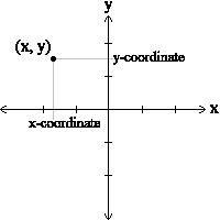
Some of the typical operations that one associates with points might be calculating the distance of a point from the origin, or from another point, or finding a midpoint of two points, or asking if a point falls within a given rectangle or circle. We'll shortly see how we can organise these operations together with the data.
A natural way to represent a point in Python is with two numeric values. The question, then, is how to group these two values into a compound object. The quick and dirty solution is to use a tuple, for example we could write p = (0,0) and q = (1,1), and for some applications that might be a good choice. But we would still need to define dedicated procedures to do something useful with these tuples representing points.
An alternative is to define a new class. This approach involves a bit more effort, but its many advantages will become apparent soon. Since we want each of our points to have an x and a y value, our first class definition looks like this:
class Point: """ The Point class represents and manipulates x,y coordinates. """ def __init__(self): """ Create a new point at the origin """ self.x = 0 self.y = 0
Although class definitions like the one above can appear anywhere in a program, they are usually put near the beginning (after the import statements). Some programmers and languages prefer to put every class in a file or module of its own --- we won't do that for now. The syntax rules for a class definition are the same as for other compound statements. There is a header which begins with the keyword, class, followed by the name of the class, and ending with a colon. Indentation levels tell us where the class ends.
If the first line after the class header is a string, it becomes the [docstring] of the class, and will be recognised by various tools. (This is also the way docstrings work in functions.)
Every class should have an initialiser method which is automatically called whenever a new object (also known as instance) of that class is created (in what follows we will use the terms object and instance interchangeably). This initialiser method has a special name __init__ (with a double underscore character before and after the name). For the class Point, the __init__ method sets the x and y coordinates of the created object to zero. In general, the __init__ method gives a programmer the opportunity to set up the attributes required within a new instance of the class by giving them their initial state/values. The self parameter (we could choose any other name, but self is the convention) is automatically set to reference the newly created object that needs to be initialised. So, for example, self.x = 0 will assign the value of 0 to the x attribute of the newly created point object itself.
We can use our new Point class now to create two Point objects:
p = Point() # Instantiate an object of type Point q = Point() # Make a second point object print(p.x, p.y, q.x, q.y) # Each point object has its own x and y
This program prints:
0 0 0 0
because during the initialisation of the objects p and q, we created two attributes called x and y for each, and gave them both the value 0.
This way of creating objects should look familiar to you. We've used classes before to create multiple Turtle objects:
from turtle import Turtle tess = Turtle() # Instantiate an object of type Turtle alex = Turtle() # Instantiate a second object of type Turtle
The variables p and q above are assigned references to two new Point objects. A function like Turtle() or Point() that creates a new object instance from its corresponding class is called a constructor. Every class automatically provides a constructor function which is named the same as the class.
It may be helpful to think of a class as a factory for making objects. The class itself isn't an instance of a point, but it contains the machinery to make point instances. Every time we call the constructor, we're asking the factory to make us a new object. As the object comes off the production line, its initialisation method is executed to get the object properly set up with its default factory settings.
The combined process of "construct me a new object" and "get its settings initialised to the factory default settings" is called instantiation.
Attributes
Object instances have both attributes (the data contained in the instance) and methods (the operations that act on that data). Whereas the methods are the same for all objects of a same class (we will see in a next section how to define such methods), the attribute values are specific to each particular instance of that class. For that reason, the attributes are sometimes also referred to as instance variables. Of course, initially they are initialised to the same factory default settings, but once an object has been created, we can modify its attribute values by using the following dot notation:
>>> p.x = 3 >>> p.y = 4
This sets the x attribute of the object instance p to the value 3 and its y attribute to the value 4.
Both modules and instances create their own namespaces, and the syntax for accessing names contained in each, called attributes, is the same. In this case the attribute we are selecting is a data item from an instance.
The following memory diagram shows the result of these assignments:
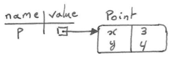
The variable p refers to a Point object, which contains two attributes x and y. Each attribute contains a number.
We can access the value of an attribute using the same syntax:
>>> print(p.y) 4 >>> x = p.x >>> print(x) 3
The expression p.x means, "Go to the point object that p refers to and get the value of its attribute named x". In this case, we assign that value to a global variable named x. There is no conflict between the variable named x (in the global namespace) and the attribute named x (in the namespace belonging to the instance). The purpose of the dot notation is to fully qualify which variable we are referring to unambiguously.
We can use dot notation as part of any expression, so the following statements are legal:
print("(x={0}, y={1})".format(p.x, p.y)) distance_from_origin = pow(p.x * p.x + p.y * p.y,1/2) print(distance_from_origin)
The first line outputs (x=3, y=4). (Note that the first line is equivalent to writing print("(x="+str(p.x)+", y="+str(p.y)+")") but uses the [format] method which supports advanced string formatting.) The second line calculates the value 5. The third line prints this calculated value.
Improving the initialiser
To create a new point object at position (7, 6) we currently need three lines of code:
p = Point() # Create a new instance of class Point p.x = 7 # Set its x attribute to the value 7 p.y = 6 # Set its y attribute to the value 6
We can make our class constructor more general by placing extra parameters into the __init__ method, as shown in this example:
class Point: """ The Point class represents and manipulates x,y coordinates. """ def __init__(self, x=0, y=0): """ Create a new point at coordinates x, y. @pre: x and y are numbers (if not supplied, the number 0 will be used) @post: the attributes x and y of this point instance have been initialised to the values x and y passed as arguments """ self.x = x self.y = y # Other statements outside the class continue below here.
The x and y parameters here are both optional. If the caller does not supply any arguments for x and y, they'll get the default values of 0. Here is our improved class in action:
>>> p = Point(4, 2) >>> q = Point(6, 3) >>> r = Point() # r represents the origin (0, 0) >>> print(p.x, q.y, r.x) 4 3 0
Below you can find another memory diagram depicting the three objects that have been created in the computer's memory.
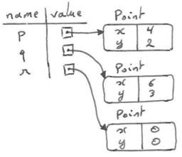
Technically speaking ...
If we are really fussy, we would argue that the __init__ method's docstring is inaccurate. Indeed, __init__ doesn't create the object (i.e. set aside memory for it; it's the constructor that does that), --- it just initialises the object to its factory-default settings after its creation.
But programming tools like for example PyScripter understand that instantiation --- creation and initialisation --- happen together, and they choose to display the initialiser's docstring as the tooltip to guide the programmer that calls the class constructor.
So we're writing the docstring so that it makes the most sense when it pops up to help the programmer who is using our Point class:
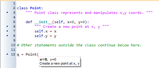
Adding other methods to the class
The key advantage of using a class like Point rather than a simple tuple (6, 7) now becomes apparent. We can add methods to the Point class that are sensible operations for points, but which may not be appropriate for other tuples like (25, 12) which might represent, say, a day and a month, e.g. Christmas day. So being able to calculate the distance from the origin is sensible for points, but not for (day, month) data. For (day, month) data, we'd like different operations, perhaps to find what day of the week it will fall on in 2050.
Creating a class like Point brings an exceptional amount of "organisational power" to our programs, and to our thinking. We can group together the sensible operations, and the kinds of data they apply to, and each instance of the class can have its own individual state.
A method behaves like a function except that it is invoked on a specific instance, e.g. t.right(90) which turns a Turtle object t 90 degrees to the right. Like data attributes, methods are accessed using the dot notation.
instance methods versus class methods
Technically speaking, there exist two kinds of methods in Python: instance methods, which can be invoked on specific instances (i.e., objects), and class methods, which can be invoked on a class itself without having to create an instance of that class first. Since most of the methods you will encounter will be instance methods, for now, when we use the term method, we mean instance method. We will not explain the notion of class methods yet, in order not to confuse you more than necessary.
Let's add another method, distance_from_origin, to our class Point to see better how methods work:
class Point: """ The Point class represents and manipulates x,y coordinates. """ def __init__(self, x=0, y=0): """ Create a new point at coordinates x, y. @pre: x and y are numbers (if not supplied, the number 0 will be used) @post: the attributes x and y of this point instance have been initialised to the values x and y passed as arguments """ self.x = x self.y = y def distance_from_origin(self): """ Compute my distance from the origin @pre: - @post: returns the Euclidian distance of this point to the origin (0,0) """ return pow((self.x ** 2) + (self.y ** 2),1/2)
When defining a method, it must always have a first parameter that refers to the instance being manipulated, i.e. the object itself. For that reason it is customary to name this parameter self.
Now let's create a few point instances, look at their attributes, and call our new distance calculation method on them. (Note that we must execute our new class definition above first, to make our modified Point class available to the interpreter.)
>>> p = Point(3, 4) >>> p.x 3 >>> p.y 4 >>> p.distance_from_origin() 5.0 >>> q = Point(5, 12) >>> q.x 5 >>> q.y 12 >>> q.distance_from_origin() 13.0 >>> r = Point() >>> r.x 0 >>> r.y 0 >>> r.distance_from_origin() 0.0
Notice that, although the method distance_from_origin(self) was defined with a first parameter self, the caller of distance_from_origin() does not explicitly supply an argument to match this self parameter; nevertheless this parameter will be bound to self automatically, behind our back. Remember that: when you define a method in a class you should add a first parameter self representing the instance being manipulated; when calling the method you should drop that parameter, it will be filled in automatically behind your back.
Instances as arguments and parameters
We can pass any object as an argument in the usual way. We've already seen this in some of the turtle examples, where we passed the turtle to some function, so that the function could control and use whatever turtle instance we passed to it. Be aware that a variable only holds a reference to an object, so passing a turtle object into a function creates an alias: both the caller and the called function now have a reference to that turtle, but there is only one turtle!
Here is a simple function involving our new Point objects:
def print_point(pt): print("({0}, {1})".format(pt.x, pt.y))
print_point takes a point as argument and formats the output in whichever way we choose. If we call print_point(p) with point p as defined previously, the output is (3, 4).
Converting an instance to a string
However, an object-oriented programmer would not do what we've just done with print_point. Rather than having a globally defined print function outside of the class definition, when working with classes and objects, a preferred alternative is to add a new method to the class definition. And we don't like chatterbox methods that call print. A better approach is to have a method so that every instance can produce a string representation of itself. This string representation can then easily be printed from the outside. Let's call this method that produces a string representation of an object to_string:
class Point: # ... same as before ... def to_string(self): return "({0}, {1})".format(self.x, self.y)
Again, observe how the method to_string takes a parameter self as first argument. Also observe how the point's attributes are accessed within that method by referring to self using the dot notation.
(As a reminder, the statement "({0}, {1})".format(self.x, self.y) is equivalent to writing "("+str(self.x)+", "+str(self.y)+")".)
Now we can say:
>>> p = Point(3, 4) >>> print(p.to_string()) (3, 4)
But doesn't there already exist a str type converter that can turn an object into a string? Yes! And doesn't print automatically use this when printing things? Yes again! But these automatic mechanisms do not (yet) seem to do exactly what we want:
>>> str(p) '<__main__.Point object at 0x01F9AA10>' >>> print(p) '<__main__.Point object at 0x01F9AA10>'
Rather than printing the contents of the object they print a unique reference to the object.
Luckily Python has a clever trick to fix this. If we call our new method __str__ (with a double underscore character before and after the method name) instead of to_string, the Python interpreter will use our code instead of the default str function whenever it needs to convert a Point to a string. Let's re-do this again, now:
class Point: # ... same as before ... def __str__(self): # All we have done is renamed the method return "({0}, {1})".format(self.x, self.y)
and now things are looking great!
>>> str(p) # Python now magically uses the __str__ # method that we wrote. (3, 4) >>> print(p) (3, 4)
Such special methods like __str__ (and also the __init__ method introduced before) are called [magic_methods] in Python. Typically, whenever you define your own new classes, you may want to implement such an __str__ method on them, to be able to easily inspect objects of those classes by printing them.
Instances as return values
Functions and methods can return object instances. For example, given two Point objects, find their midpoint. First we'll write this as a regular function:
def midpoint(p1, p2): """ @pre: p1 and p2 are instances of class Point @post: returns the midpoint of points p1 and p2 """ mx = (p1.x + p2.x)/2 my = (p1.y + p2.y)/2 return Point(mx, my)
This function creates and returns a new Point object:
>>> p = Point(3, 4) >>> q = Point(5, 12) >>> r = midpoint(p, q) >>> print(r) (4.0, 8.0)
However, as mentioned before, an object-oriented programmer would prefer to define this as a method defined on the class, rather than as a globally defined function. So, let us try to write this function as a method instead. Suppose we have a point object, and wish to find the midpoint halfway between itself and some other target point:
class Point: # ... def halfway(self, target): """ @pre: target is an instance of class Point @post: returns a new instance of class Point representing the halfway point between myself and the target """ mx = (self.x + target.x)/2 my = (self.y + target.y)/2 return Point(mx, my)
This method is almost identical to the function, aside from some renaming. It's usage might be like this:
>>> p = Point(3, 4) >>> q = Point(5, 12) >>> r = p.halfway(q) >>> print(r) (4.0, 8.0)
While this example assigns each point to a variable, this need not be done. Just as function calls are composable, method calls and object instantiation are also composable, leading to this alternative that uses no variables:
>>> print(Point(3, 4).halfway(Point(5, 12))) (4.0, 8.0)
A change of perspective
The original syntax for a function call, print_time(current_time), suggests that the function is the active agent. It says something like, "Hey, print_time! Here's an object for you to print."
In object-oriented programming, objects are considered the active agents instead. An invocation like current_time.print_time() says "Hey current_time! Please print yourself!"
In our early introduction to turtles, we used an object-oriented style, so that we said t.forward(100), which asks the turtle t to move itself forward by the given number of steps.
This change in perspective might be more polite, but it may not initially be obvious that it is useful. But sometimes shifting responsibility from the functions onto the objects makes it possible to write more versatile functions, and makes it easier to maintain and reuse code.
The most important advantage of the object-oriented style is that it fits our mental chunking and real-life experience more accurately. In real life our cook method is part of our microwave oven --- we don't have a cook function sitting in the corner of the kitchen, into which we pass the microwave! Similarly, we use the cellphone's own methods to send an sms, or to change its state to silent. The functionality of real-world objects tends to be tightly bound up inside the objects themselves. [object_oriented_programming] allows us to accurately mirror this when we organise our programs.
Objects can have state
Objects are most useful when we also need to keep some state that is updated from time to time. Consider a turtle object. Its state consists of things like its position, its heading, its colour, and its shape. A method like left(90) updates the turtle's heading, forward changes its position, and so on.
For a bank account object, a main component of the state would be the current balance, and perhaps a log of all transactions. The methods would allow us to query the current balance, deposit new funds, or make a payment. Making a payment would include an amount, and a description, so that this could be added to the transaction log. We'd also want a method to show the transaction log.
Glossary
- attribute
- One of the named data items that makes up an object. Another word for attribute is instance variable.
- class
- A user-defined compound type. A class can also be thought of as a template or factory for the objects that are instances of it.
- constructor
- A class can also be seen as a "factory" for making objects of a certain kind. Every class thus provides a constructor method, called by the same name as the class, for making new instances of this kind. If the class has an initialiser method, this method is used to get the attributes (i.e. the state) of the new instance properly set up.
- initialiser method
- A special method in Python (called __init__) that is invoked automatically to set a newly created object's attributes to their initial (factory-default) state.
- instance
- An object whose type is of some class. The words instance and object are used interchangeably.
- instance variable
- Since the attribute values of an object are specific to that particular object (i.e., another object of the same class may have another value for that attribute), they are sometimes also referred to as instance variables.
- instantiate
- To create an instance of a class, and to run its initialiser method.
- instance method
- A function that is defined inside a class definition and is invoked on instances of that class.
- magic method
- Magic methods are special methods like __init__ or __str__ that you can define to add some magic to your classes. For example Python magically knows that when a new object gets constructed it should call the __init__ method to initialise the attributes of the newly created object, or that when you print an object, it should call the __str__ method to get a printable string representation of the object. Magic methods are always surrounded by double underscores.
- method
- If it is clear from the context we will often refer to an instance method simply as a method. (We will learn later that there is also such a thing as class methods, which is not the same as instance methods.)
- object
- A compound data type that is often used to model a thing or concept in the real world. It bundles together the data and the operations that are relevant for that kind of data. The words instance and object are used interchangeably.
- object-oriented programming
- A powerful style of programming in which data and the operations that manipulate it are organized into objects.
- object-oriented language
- A language that provides features, such as user-defined classes and inheritance, that facilitate object-oriented programming.
References
| [ThinkCS] | How To Think Like a Computer Scientist --- Learning with Python 3 |
| [object_oriented_programming] | (1, 2) http://en.wikipedia.org/wiki/Object-oriented_programming |
| [programming_paradigm] | http://en.wikipedia.org/wiki/Programming_paradigm |
| [procedural_programming] | http://en.wikipedia.org/wiki/Procedural_programming |
| [magic_methods] | https://rszalski.github.io/magicmethods/ |
| [docstring] | https://www.python.org/dev/peps/pep-0257/ |
| [format] | https://www.python.org/dev/peps/pep-3101/#id16 |
Classes and Objects – Digging a little deeper
Source: this section is heavily based on Chapter 16 of [ThinkCS] though adapted to better fit with the contents, terminology and notations of this particular course.
Rectangles
Suppose we want a class to represent rectangles located somewhere in the Cartesian X-Y plane. What information do we have to provide in order to specify such a rectangle? To simplify things, let us assume that the rectangle is always oriented either vertically or horizontally, never at an angle.
There are a few possibilities: we could specify the center of the rectangle (two coordinates) and its size (width and height); or we could specify one of the corners and the size; or we could specify two opposing corners. A conventional choice is to specify the upper-left corner of the rectangle, and its size.
As with the Point class before, we'll define a new class Rectangle, and provide it with an initialiser method __init__ and a string converter method __str__. Also don't forget to always add as first parameter to your methods a reference to self.
class Rectangle: """ The Rectangle class represents rectangles in a Cartesian plane. """ def __init__(self, pos, w, h): """ Create a new rectangle with upper-left corner at point pos, with width w and height h. @pre: pos is an instance of class Point width and height are positive numbers @post: the attributes corner, width and height of this rectangle instance have been initialised to the values pos, w and h passed as arguments """ self.corner = pos self.width = w self.height = h def __str__(self): """ @pre: - @post: returns a string representation of this rectangle in the following format ((x, y), width, height) where width and height are the values of the corresponding attributes of this object and x and y are the corresponding attributes of the point object stored in the corner attribute """ return "({0}, {1}, {2})".format(self.corner, self.width, self.height) box = Rectangle(Point(0, 0), 100, 200) bomb = Rectangle(Point(100, 80), 5, 10) # In some video game print("box: ", box) print("bomb: ", bomb)
Note how, to specify the upper-left corner, we embedded a Point object (as was defined in the previous section) within our new Rectangle object. We create two new Rectangle objects, and then print them, which produces:
box: ((0, 0), 100, 200) bomb: ((100, 80), 5, 10)
The dot operator can be composed (chained). For example, the expression box.corner.x means: "Go to the object that box refers to, select its attribute named corner, then go to that object and select its attribute named x".
The figure below shows the state of this object:
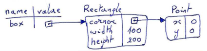
From the figure it can easily be seen that printing box.corner.x would produce:
>>> print(box.corner.x) 0
When reasoning about the state of objects (their attributes and the values they contain), we strongly encourage you to draw such memory diagrams.
Objects are mutable
We can change the state of an object by making an assignment to one of its attributes. For example, to grow the size of a rectangle without changing its position, we could modify the values of its width and height attributes:
box.width += 50 box.height += 100
The memory diagram below sketches the effect of making these modifications (in green):
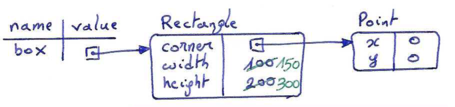
After this, print("box: ", box) produces as output:
box: ((0, 0), 150, 300)
However, we prefer to provide a method to encapsulate this state change operation inside the class. We will also provide another method to move the position of the rectangle over a certain distance:
class Rectangle: # ... same as before ... def grow(self, delta_width, delta_height): """ Grow (or shrink) this rectangle by the deltas @pre: delta_width and delta_height are (positive or negative) numbers @post: this rectangle's width was grown to its original width plus delta_width (or shrunk in case delta_width is negative); this rectangle's height was grown to its original height plus delta_height (or shrunk in case delta_height is negative); nothing is returned """ self.width += delta_width self.height += delta_height def move(self, dx, dy): """ Move this object by the given distances @pre: dx and dy are (positive or negative) numbers @post: the x-coordinate of this rectangle's corner was moved from its original position x to x plus dx (moved right if dx is positive or moved left if dx is negative); the y-coordinate of this rectangle's corner was moved from its original position y to y plus dy (moved down if dy is positive or moved up if dy is negative); nothing is returned """ self.corner.x += dx self.corner.y += dy
Let us try this:
>>> r = Rectangle(Point(10,5), 100, 50) >>> print(r) ((10, 5), 100, 50) >>> r.grow(25, -10) >>> print(r) ((10, 5), 125, 40) >>> r.move(-10, 10) print(r) ((0, 15), 125, 40)
Again, a memory diagram may help you to better visualise how the state of the rectangle and point objects get modified (the part in blue corresponds to the definition of the rectangle object, in pink the effect of growing it, in green the effect of moving it):
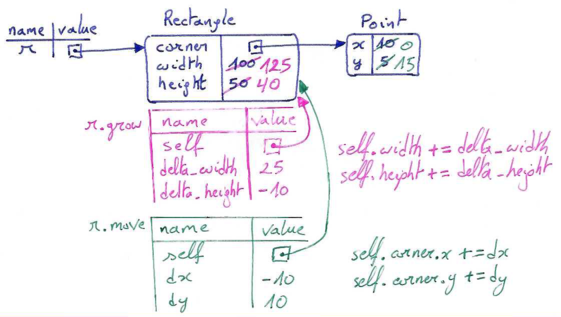
Sameness
The meaning of the word "same" seems perfectly clear until we give it some thought, and then we realize there is more to it than we initially expected.
For example, if we say, "Alice and Bob have the same mother", we mean that her mother and his are the same person. If we say, however, "Alice and Bob have the same car", we probably mean that her car and his are the same make and model, but that they are two different cars. But if we say, "Alice and Bob share the same car", we probably mean that they actually share the usage of a single car.
When we talk about objects, there is a similar ambiguity. For example, if two Points are the same, does that mean they are two point objects that contain the same data (coordinates) or that they are actually the same object?
We can use the is operator to find out if two references refer to the same object:
>>> p1 = Point(3, 4) >>> p2 = Point(3, 4) >>> p1 is p2 False
In this example, even though p1 and p2 contain the same coordinates, they are not the same object. If we assign the value of p1 to a new variable named p3, however, then the two variables are aliases of (refer to) the same object:
>>> p3 = p1 >>> p1 is p3 True
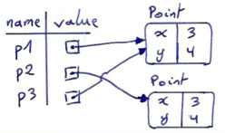
This type of equality is called shallow equality because it compares only the references, not the actual contents of the objects' attributes. With the is operator, two things are considered the same only if they refer to the exact same thing. This means that even the following comparison would yield False:
>>> Point(3, 4) is Point(3, 4) False
The reason is that whenever you call the Point(3, 4) constructor you create a new distinct point object that happens to have the values 3 and 4 for its x and y coordinates. But the two objects are distinct and stored in different memory locations.
To compare the contents of the objects — deep equality — we can write a function called same_coordinates:
def same_coordinates(p1, p2): """ @pre: p1 and p2 are instances of class Point @post: returns True if both the x attribute of p1 and p2 are equal and their y attributes are equal; returns False otherwise """ return (p1.x == p2.x) and (p1.y == p2.y)
Now if we try to run the comparisons above again, but using same_coordinates as a comparator rather than the is operator, we can see that they are all considered the same:
>>> same_coordinates(p1, p2) True >>> same_coordinates(p1, p3) True >>> same_coordinates(Point(3, 4),Point(3, 4)) True
Of course, if two variables refer to the same object (as is the case with p1 and p3), they have both shallow and deep equality.
Beware of ==
Python has a powerful feature that allows a designer of a class to decide what an operation like == or < should mean. We'll cover that in more detail later, but the principle is the same as how we can control how our own objects are converted to strings, as was illustrated in the previous section with the magic method __str__. But sometimes the language implementors will attach a shallow equality semantics to ==, and sometimes deep equality, as shown in this little experiment:
p1 = Point(4, 2) p2 = Point(4, 2) print("== on Points returns", p1 == p2) # By default, == on Point objects does a SHALLOW equality test l1 = [2,3] l2 = [2,3] print("== on lists returns", l1 == l2) # But by default, == does a DEEP equality test on lists
This outputs:
== on Points returns False == on lists returns True
So we conclude that even though the two lists (or tuples, etc.) are distinct objects with different memory addresses, for lists the == operator tests for deep equality, while in the case of points it makes a shallow test.
Copying
Aliasing (different variables referring to a same object) can make a program difficult to read because changes made in one place might have unexpected effects in another place. It is hard to keep track of all the variables that might refer to a given object.
Copying an object is often an alternative to aliasing. The copy module contains a function called copy that can duplicate any object:
>>> import copy >>> p1 = Point(3, 4) >>> p2 = copy.copy(p1) >>> p1 is p2 False >>> same_coordinates(p1, p2) True
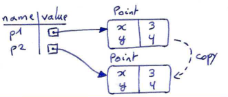
Once we import the copy module, we can use the copy function to make a new Point. p1 and p2 are not a reference to the same object, but they are distinct point objects that contain the same data. p2 is a newly created object of which the data is copied from p1.
To copy a simple object like a Point, which doesn't contain any embedded objects, using the copy function suffices, even though it only performs a shallow copying.
For something like a Rectangle object, which contains an internal reference to a Point object (to represent its upper-left corner), a simple shallow copy wouldn't suffice however. It would create a new Rectangle object, copying the values of the width and height attributes of the original Rectangle object. But for the corner attribute it would simply copy the reference to the Point object it contains, so that both the old and the new Rectangle's corner attribute would refer to the same Point.
>>> import copy >>> b1 = Rectangle(Point(0, 0), 100, 200) >>> b2 = copy.copy(b1)
If we create a rectangle b1 in the usual way, and then make a copy b2, using copy, the resulting memory diagram looks like this:
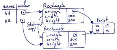
This is almost certainly not what we want. In this case, invoking grow on one of the Rectangle objects would not affect the other (since the grow method only acts on the width and height attributes which were copied), but invoking move on either Rectangle object would affect the other! That would be very weird, since the rectangles would share their upper-left corner but not their size attributes.
>>> b1.move(10,10) >>> print(b2.corner) (10,10)
In the example above, although we didn't explicitly move b2, we can see that its corner object has changed as a side-effect of moving b1. This behavior is confusing and error-prone. The problem is that the shallow copy of the rectangle object has created an alias to the Point that represents the corner, rather than making a copy of that point.
Fortunately, the copy module also contains a function named deepcopy that copies not only the object but also any embedded objects (recursively). It won't be surprising to learn that this operation is called a deep copy.
>>> b1 = Rectangle(Point(0, 0), 100, 200) >>> b2 = copy.deepcopy(b1) >>> b1.move(10,10) >>> print(b1.corner) (10,10) >>> print(b2.corner) (0,0)
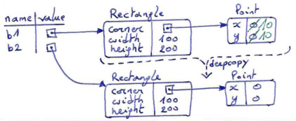
Now b1 and b2 are completely separate objects.
Glossary
- deep copy
- To copy the contents of an object as well as any embedded objects, and any objects embedded in them, and so on; implemented by the deepcopy function in the copy module.
- deep equality
- Equality of values, or two references that point to (potentially different) objects that have the same attribute values.
- shallow copy
- To copy the contents of an object, including any references to embedded objects; implemented by the copy function in the copy module.
- shallow equality
- Equality of references, or two references that point to the same object.
- string converter method
- A magic method in Python (called __str__) that produces an informal string representation of an object. For example, this is the string that will be printed when calling the print function on that object.
References
| [ThinkCS] | How To Think Like a Computer Scientist --- Learning with Python 3 |
Even more object-oriented programming
Source: this section is heavily based on the first half of Chapter 21 of [ThinkCS] though adapted to better fit with the contents, terminology and notations of this particular course.
Now that we've seen the basics of object-oriented programming and have created our own first Point and Rectangle classes, let's take things yet a step further.
MyTime
As another example of a user-defined class, we'll define a class called MyTime that records the time of day. We provide an __init__ method to ensure that every instance is created with appropriate attributes and initialisation. The class definition looks like this:
class MyTime: def __init__(self, hrs=0, mins=0, secs=0): """ @pre: hrs, mins, secs are positive integers; 0 <= mins < 60, 0 <= secs < 60; if not supplied a default value of 0 is used @post: the attributes hours, minutes and seconds of this MyTime object have been initialised to hrs, mins, secs (or 0 if no values were supplied) """ self.hours = hrs self.minutes = mins self.seconds = secs
We can then create and instantiate a new MyTime object by calling the constructor with the necessary arguments for the initialisation method:
tim1 = MyTime(11, 59, 30)
The memory diagram for this object looks like this:
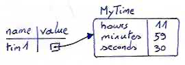
We leave it as an exercise for the reader (please do it!) to also add a __str__ method so that MyTime objects can print themselves decently. For example, the object above should print as 11:59:30. (If you don't know how to do this, look at the Rectangle class of the previous chapter for inspiration.)
Pure functions
In the next few sections, we'll write two versions of a function called add_time, which calculates the sum of two MyTime objects. They will demonstrate two kinds of functions: pure functions and modifiers.
The following is a first rough version of add_time:
def add_time(t1, t2): """ @pre: t1 and t2 are instances of class MyTime @post: a new MyTime object is returned of which the hours, minutes and seconds attributes are the sum of the respective attributes in t1 and t2 """ h = t1.hours + t2.hours m = t1.minutes + t2.minutes s = t1.seconds + t2.seconds sum_t = MyTime(h, m, s) return sum_t
The function creates a new MyTime object and returns a reference to the new object. This is called a pure function because it does not modify any of the objects passed to it as parameters and it has no side effects, such as updating global variables, displaying a value, or getting user input.
Here is an example of how to use this function. We'll create two MyTime objects: current_time, which contains the current time; and bread_time, which contains the amount of time it takes for a breadmaker to make bread. Then we'll use add_time to figure out when the bread will be done.
>>> current_time = MyTime(9, 14, 30) >>> bread_time = MyTime(3, 35, 0) >>> done_time = add_time(current_time, bread_time) >>> print(done_time) 12:49:30
The output of this program is 12:49:30, which is correct. On the other hand, there are cases where the result is not correct. Can you think of one?
The problem is that this function does not deal with cases where the number of seconds or minutes adds up to more than sixty. When that happens, we have to carry the extra seconds into the minutes column or the extra minutes into the hours column.
Here's an improved version of the function. (We left out its specification, because it would get pretty big and we will soon propose a better alternative solution.)
def add_time(t1, t2): h = t1.hours + t2.hours m = t1.minutes + t2.minutes s = t1.seconds + t2.seconds if s >= 60: s -= 60 m += 1 if m >= 60: m -= 60 h += 1 sum_t = MyTime(h, m, s) return sum_t
This function is already starting to get bigger, and still doesn't work for all possible cases. Later we will suggest an alternative approach that yields better code.
Modifiers
There are times when it is useful for a function to modify one or more of the objects it gets as parameters. Usually, the caller keeps a reference to the objects it passes, so any changes the function makes are visible to the caller. Functions that work this way are called modifiers.
For example, increment, which adds a given number of seconds to a MyTime object, when written as a modifier, could behave like this:
>>> t = MyTime(10,20,30) >>> increment(t,70) >>> print(t) 10:21:40
A rough draft of the implementation of this function looks like this:
def increment(t, secs): """ @pre: t is an instance of MyTime; secs is a positive integer @post: the seconds attribute of t is modified by adding secs; if the amount of seconds in t becomes > 60, each surplus of 60 seconds spills over to an extra minute added to the minutes attribute of t; if the amount of minutes in t becomes > 60, each surplus of 60 minutes spills over to an extra hour added to the hours attribute of t; nothing is returned """ t.seconds += secs if t.seconds >= 60: t.seconds -= 60 t.minutes += 1 if t.minutes >= 60: t.minutes -= 60 t.hours += 1
The first line performs the basic operation; the remainder deals with the special cases we saw before.
Note that this function has no return statement nor does it need to create a new object. It simply modifies the state of the Time object t that was passed as first parameter to the function.
Is this function correct? What happens if the parameter secs is much greater than sixty? In that case, it is not enough to carry once; we have to keep doing it until t.seconds is less than sixty. One solution is to replace the if statements with while statements:
def increment(t, secs): # SAME SPECIFICATION AS BEFORE t.seconds += secs while t.seconds >= 60: t.seconds -= 60 t.minutes += 1 while t.minutes >= 60: t.minutes -= 60 t.hours += 1
This function is now correct when seconds is not negative, but it is still not a particularly good nor efficient solution.
>>> t = MyTime(10,20,30) >>> increment(t,100) >>> print(t) 10:22:10
Converting increment to a method
Once again, since object-oriented programmers would prefer to put functions that work with MyTime objects directly into the MyTime class, let's convert increment to a method. To save space, we will leave out previously defined methods in that class, but you should keep them in your version:
class MyTime: # Previous method definitions here... def increment(self, seconds): # SAME SPECIFICATION AS BEFORE self.seconds += seconds while self.seconds >= 60: self.seconds -= 60 self.minutes += 1 while self.minutes >= 60: self.minutes -= 60 self.hours += 1
The transformation is purely mechanical: we move the definition into the class definition and change the name of the first parameter (and all occurrences of that parameter in the method body) to self, to fit with Python style conventions.
Now we can invoke increment using the dot syntax for invoking a method, instead of writing increment(current_time,500) :
>>> current_time = MyTime(11, 58, 30) >>> current_time.increment(500) >>> print(current_time) 12: 6:50
The object current_time on which the method is invoked gets assigned to the first parameter, self. The second parameter, seconds gets the value 500.
An "Aha!" moment
An "Aha!" moment is that moment or instant at which the solution to a problem suddenly becomes clear. Often a high-level insight into a problem can make the programming much easier.
A three-digit number in base 10, for example the number 284, can be represented by 3 digits, the right most one (4) representing the units, the middle one (8) representing the tens, and the left-most one representing the hundreds. In other words, 284 = 2*100 + 8*10 + 4*1.
Our "Aha!" moment consists of the insight that a MyTime object is actually a three-digit number in base 60 ! The "seconds" correspond to the units, the "minutes" to the sixties, and the hours to the thirty-six hundreds. Indeed, 12h03m30s corresponds to 12*3600 + 3*60 + 30 = 43410 seconds.
When we were writing the add_time and increment functions and methods, we were effectively doing addition in base 60, which explains why we had to carry over remaining digits from one column to the next.
This observation suggests another approach to the entire problem --- we can convert a MyTime object into a single number (in base 10, representing the seconds) and take advantage of the fact that the computer knows how to do arithmetic with numbers. The following method can be added to the MyTime class to convert any instance into a corresponding number of seconds:
class MyTime: # ... def to_seconds(self): """ @pre: - @post: returns the total number of seconds represented by this instance of MyTime """ return self.hours * 3600 + self.minutes * 60 + self.seconds
>>> current_time = MyTime(11, 58, 30) >>> seconds = current_time.to_seconds() >>> print(current_time) 11:58:30 >> print(seconds) 43110
Now, all we need is a way to convert from an integer, representing the time in seconds, back to a MyTime object. Supposing we have tsecs seconds, some integer division and modulus operators can do this for us:
hrs = tsecs // 3600 leftoversecs = tsecs % 3600 mins = leftoversecs // 60 secs = leftoversecs % 60
You might have to think a bit to convince yourself that this technique to convert from one base to another is correct. Remember that the // operator represents integer division and that the modulus operator % calculates the remainder of integer division.
As mentioned in the previous sections, one of the main goals of object-oriented programming is to wrap together data with the operations that apply to it. So we'd like to put the above conversion logic inside the MyTime class. A good solution is to rewrite the class initialisation method __init__ so that it can cope with initial values of seconds or minutes that are outside the normalised values. (A normalised time would be something like 3 hours 12 minutes and 20 seconds. The same time, but unnormalised could be 2 hours 70 minutes and 140 seconds, where the minutes or seconds are more than the expected maximum of 60.)
Let's rewrite a more powerful initialiser for MyTime:
class MyTime: # ... def __init__(self, hrs=0, mins=0, secs=0): """ Create a new MyTime object initialised to hrs, mins, secs. @pre: hrs, mins, secs are positive integers; if not supplied a default value of 0 is used @post: the attributes hours, minutes and seconds of this MyTime object have been initialised to hrs, mins, secs (or 0 if no values were supplied) In case the values of mins and secs are outside the range 0-59, the resulting MyTime object will be normalised, so that they are in this range """ # Calculate the total number of seconds to represent totalsecs = hrs*3600 + mins*60 + secs self.hours = totalsecs // 3600 # Split in h, m, s leftoversecs = totalsecs % 3600 self.minutes = leftoversecs // 60 self.seconds = leftoversecs % 60
Now we can rewrite add_time like this:
def add_time(t1, t2): """ @pre: t1 and t2 are instances of class MyTime @post: a new MyTime object is returned of which the total time in seconds is the sum of the total time in seconds of t1 and t2 """ secs = t1.to_seconds() + t2.to_seconds() return MyTime(0, 0, secs)
This version is much shorter than the original, and it is much easier to demonstrate or reason that it is correct. Notice that we didn't have to do anything for carrying over seconds or minutes that are too large; that is handled automatically by our new initialiser method now. (Isn't that just wonderful?)
>>> current_time = MyTime(9, 14, 30) >>> bread_time = MyTime(3, 35, 0) >>> done_time = add_time(current_time, bread_time) >>> print(done_time) 12:49:30
Note that we could also implement add_time as a method defined on the class MyTime rather than as a globally defined function, but we will leave that to the next chapter.
The final question that remains now is how we can rewrite the increment method that we wrote before, without having to reimplement the logic that we now put into our new initialiser method. The answer to this question is in the question. What if we simply try to call the __init__ method from within the increment method so as to reuse its logic. This can be done surprisingly easily:
def increment(self, secs): """ @pre: t is an instance of MyTime; secs is a positive integer @post: the seconds attribute of t is modified by adding secs; if necessary t gets normalized so that neither the amount of seconds in t nor the amount of minutes in t becomes > 60; nothing is returned """ self.__init__(self.hours,self.minutes,self.seconds+secs)
Again, the carrying over of seconds or minutes that are too large is handled automatically by the initialiser method. It is important to observe that, as opposed to the add_time method, we are not creating a new MyTime object here. We are simply calling __init__ to assign a new state to the existing instance (self).
>>> current_time = MyTime(11, 58, 30) >>> current_time.increment(500) >>> print(current_time) 12: 6:50
Generalisation
In some ways, converting from base 60 to base 10 and back is harder than just dealing with time. Base conversion is more abstract; our intuition for dealing with time is better.
However, if we have the insight to treat time objects as base 60 numbers and make the investment of writing the conversions, we get a program that is shorter, easier to read and debug, and more reliable.
It is also easier to add features later. For example, imagine subtracting two MyTime objects to find the duration between them. The naive approach would be to implement subtraction with borrowing. Using the conversion functions would be easier and more likely to be correct.
Ironically, sometimes making a problem harder (or more general) makes the programming easier, because there are fewer special cases and fewer opportunities for error.
Specialisation versus Generalisation
Computer Scientists are generally fond of specialising their types, while mathematicians often take the opposite approach, and generalise everything.
What do we mean by this?
If we ask a mathematician to solve a problem involving weekdays, days of the century, playing cards, time, or dominoes, their most likely response is to observe that all these objects can be represented by integers. Playing cards, for example, can be numbered from 0 to 51. Days within the century can be numbered. Mathematicians will say "These things are enumerable --- the elements can be uniquely numbered (and we can reverse this numbering to get back to the original concept). So let's number them, and confine our thinking to integers. Luckily, we have powerful techniques and a good understanding of integers, and so our abstractions --- the way we tackle and simplify these problems --- is to try to reduce them to problems about integers."
Computer scientists tend to do the opposite. We will argue that there are many integer operations that are simply not meaningful for dominoes, or for days of the century. So we'll often define new specialised types, like MyTime, because we can restrict, control, and specialise the operations that are possible. Object-oriented programming is particularly popular because it gives us a good way to bundle methods and specialised data into a new type. (We call such a type an abstract data type.)
Both approaches are powerful problem-solving techniques. Often it may help to try to think about the problem from both points of view --- "What would happen if I tried to reduce everything to very few primitive types?", versus "What would happen if this thing had its own specialised type?"
Glossary
- functional programming style
- A style of program design in which the majority of functions are pure.
- generalisation
- A problem-solving technique where a concrete problem gets generalised into a more abstract one that is easier to solve
- modifier
- A function or method that changes one or more of the objects it receives as parameters. Most modifier functions are void (do not return a value).
- normalized
- Data is said to be normalized if it fits into some reduced range or set of rules. We usually normalize our angles to values in the range [0..360[. We normalize minutes and seconds to be values in the range [0..60[. And we'd be surprised if the local store advertised its cold drinks at "One dollar, two hundred and fifty cents".
- pure function
- A function that does not modify any of the objects it receives as parameters. Most pure functions are not void but return a value.
- specialisation
- A problem-solving technique where a more abstract problem gets specialised into a more concrete one that is easier to solve
References
| [ThinkCS] | How To Think Like a Computer Scientist --- Learning with Python 3 |
Overloading and Polymorphism
Source: this section is heavily based on the second half of Chapter 21 of [ThinkCS] though adapted to better fit with the contents, terminology and notations of this particular course.
In the previous chapter we introduced a new class MyTime representing time objects in hours, minutes and seconds with methods like __init__, __str__, increment and to_seconds. For easy reference, we repeat the implementation of this class so far here below:
class MyTime: def __init__(self, hrs=0, mins=0, secs=0): """ Create a new MyTime object initialised to hrs, mins, secs. @pre: hrs, mins, secs are positive integers; if not supplied a default value of 0 is used @post: the attributes hours, minutes and seconds of this MyTime object have been initialised to hrs, mins, secs (or 0 if no values were supplied) In case the values of mins and secs are outside the range 0-59, the resulting MyTime object will be normalised, so that they are in this range """ # Calculate the total number of seconds to represent totalsecs = hrs*3600 + mins*60 + secs self.hours = totalsecs // 3600 # Split in h, m, s leftoversecs = totalsecs % 3600 self.minutes = leftoversecs // 60 self.seconds = leftoversecs % 60 def __str__(self) : """ @pre: - @post: returns a string representation of this MyTime object in the format "hh:mm:ss" """ return "{0:2}:{1:2}:{2:2}".format(self.hours, self.minutes, self.seconds) def increment(self, secs): """ @pre: t is an instance of MyTime; secs is a positive integer @post: the seconds attribute of t is modified by adding secs; if necessary t gets normalized so that neither the amount of seconds in t nor the amount of minutes in t becomes > 60; nothing is returned """ self.__init__(self.hours,self.minutes,self.seconds+secs) def to_seconds(self): """ @pre: - @post: returns the total number of seconds represented by this instance of MyTime """ return self.hours * 3600 + self.minutes * 60 + self.seconds
Binary operations
We will now add a few more interesting methods to this class. Let us start by an after function which compares two times, and tells us whether the first time is strictly after the second, e.g.
>>> t1 = MyTime(10, 55, 12) >>> t2 = MyTime(10, 48, 22) >>> t1.after(t2) # Is t1 after t2? True
This is slightly more complicated because it operates on two MyTime objects, not just one. But we'd prefer to write it as a method anyway, in this case, a method on the first argument. We can then invoke this method on one object and pass the other as an argument:
if current_time.after(done_time): print("The bread will be done before it starts!")
We can almost read the invocation like English: If the current time is after the done time, then...
To implement this method, we can again use our "Aha!" insight of the previous chapter and reduce both times to seconds, which yields a very compact method definition:
class MyTime: # Previous method definitions here... def after(self, other): """ @pre: other is an instance of MyTime @post: returns True if this MyTime instance (self) is strictly greater than other; returns False otherwise """ return self.to_seconds() > other.to_seconds()
This is a great way to code this: if we want to tell if the first time is after the second time, turn them both into integers and compare the integers.
Operator overloading
Some languages, including Python, make it possible to have different meanings for the same operator when applied to different types. For example, + in Python means quite different things for integers and for strings. This feature is called operator overloading.
It is especially useful when programmers can also overload the operators for their own user-defined types.
For example, to override the addition operator + for MyTime objects, we can provide a magic method named __add__:
class MyTime: # Previously defined methods here... def __add__(self, other): """ @pre: other is an instance of class MyTinme @post: a new MyTime object is returned of which the total time in seconds is the sum of the total time in seconds of t1 and t2 """ secs = self.to_seconds() + other.to_seconds() return MyTime(0, 0, secs)
As usual, the first parameter self is the MyTime object on which the method is invoked. The second parameter is conveniently named other to distinguish it from self. To add two MyTime objects, we create and return a new MyTime object that contains their sum in seconds. (Remember from the previous chapter that the __init__ method normalises MyTime objects by converting their value in seconds to hours, minutes and seconds.)
Now, when we apply the + operator to MyTime objects, Python magically invokes the __add__ method that we have written:
>>> t1 = MyTime(1, 15, 42) >>> t2 = MyTime(3, 50, 30) >>> t3 = t1 + t2 >>> print(t3) 5: 6:12
The expression t1 + t2 is equivalent to t1.__add__(t2), but obviously more elegant. As an exercise, add a method __sub__(self, other) that overloads the subtraction operator -, and try it out.
For the next couple of exercises we'll go back to the Point class defined when we first introduced objects (in chapter Classes and Objects – the Basics), and overload some of its operators. Firstly, adding two points adds their respective (x, y) coordinates:
class Point: # Previously defined methods here... def __add__(self, other): """ @pre: other is an instance of class Point @post: retuns a new instance of class Point of which the x-coordinate (resp. y-coordinate) is the sum of the x-coordinate (resp. y-coordinate) of self and other """ return Point(self.x + other.x, self.y + other.y)
>>> p = Point(3, 4) >>> q = Point(5, 7) >>> r = p + q # equivalent to r = p.__add__(q) >>> print(r) (8, 11)
There are several ways to override the behaviour of the multiplication operator *: by defining a magic method named __mul__, or __rmul__, or both.
If the left operand of * is a Point, Python invokes __mul__, which assumes that the other operand is also a Point. In this case we compute the dot product of the two Points, defined according to the rules of linear algebra:
def __mul__(self, other): """ @pre: other is an instance of class Point @post: returns the dot product of the points contained in self and other, in other words the sum of the product of their respective x- and y-coordinates """ return self.x * other.x + self.y * other.y
If the left operand of * is a primitive type and the right operand is a Point, Python invokes __rmul__, which performs scalar multiplication:
def __rmul__(self, other): """ @pre: other is a number @post: returns the scalar multiplication of the Point object contained in self with the number contained in other; in other words a new Point object of which the x- and y-coordinates are those of self, multiplied by other """ return Point(other * self.x, other * self.y)
The result is a new Point whose coordinates are a multiple of the original coordinates. If other is a type that cannot be multiplied by a floating-point number, then __rmul__ will yield an error.
This example demonstrates both kinds of multiplication:
>>> p1 = Point(3, 4) >>> p2 = Point(5, 7) >>> print(p1 * p2) 43 >>> print(2 * p2) (10, 14) >>> print(p2 * 2)
But what happens if we try to evaluate p2 * 2? Since the first parameter is a Point, Python invokes __mul__ with 2 as the second argument. Inside __mul__, the program tries to access the x coordinate of other, which fails because an integer has no attributes:
>>> print(p2 * 2) AttributeError: 'int' object has no attribute 'x'
Unfortunately, the error message is a bit opaque. This example demonstrates some of the difficulties of object-oriented programming. Sometimes it is hard enough just to figure out what code is running.
If you wonder if we could avoid this error and make __mul__ work as well when the second argument is a number, the answer is yes:
def __mul__(self, other): """ @pre: other is an instance of class Point or a number @post: IF other is a Point object, returns the dot product of the points contained in self and other, in other words the sum of the product of their respective x- and y-coordinates IF other is a number, returns the scalar multiplication of the Point object contained in self with the number contained in other """ if type(other) is Point : return self.x * other.x + self.y * other.y if (type(other) is int) or (type(other) is float) : return other * self
Polymorphism
Most of the methods we have written so far only work for a specific type. When we create a new object, we write methods that operate on that type. But there are certain operations that we may want to apply to many types, such as the arithmetic operators + and * in the previous section. If many types support the same set of operations, we can write functions that work on any of those types.
For example, the multadd operation (which is common in linear algebra) takes three parameters; it multiplies the first two and then adds the third. We can write it in Python like this:
def multadd(x, y, z): return x * y + z
This function will work for any values of x and y that can be multiplied and for any value of z that can be added to the product.
We can invoke it with numeric values:
>>> multadd(3, 2, 1) 7
but also with Point objects:
>>> p1 = Point(3, 4) >>> p2 = Point(5, 7) >>> print(multadd (2, p1, p2)) (11, 15) >>> print(multadd (p1, p2, 1)) 44
In the first case, the Point p1 is multiplied by a scalar 2 and then added to another Point p2. In the second case, the dot product of p1 and p2 yields a numeric value, so the third parameter also has to be a numeric value.
Functions like +, * and multadd that can work with arguments of different types are called polymorphic. In object-oriented programming, polymorphism (from the Greek meaning "having multiple forms") is the characteristic of being able to assign a different meaning or usage to something in different contexts. In this case, the context that varies are the types of arguments taken by the function.
As another example, consider the function front_and_back, which prints a list twice, forward and backward:
def front_and_back(front): import copy back = copy.copy(front) back.reverse() print(str(front) + str(back))
Because the reverse method is a modifier, we first make a copy of the list before reversing it. That way, this function doesn't modify the list it gets as a parameter.
Here's an example that applies front_and_back to a list:
>>> my_list = [1, 2, 3, 4] >>> front_and_back(my_list) [1, 2, 3, 4][4, 3, 2, 1]
Since we designed this function to apply to lists, of course it is not so surprising that it works. What would be surprising is if we could apply it to a Point.
To determine whether a function can be applied to a new type, we apply Python's fundamental rule of polymorphism, called the duck typing rule: If all of the operations inside the function can be applied to the type, the function can be applied to the type. The operations in the front_and_back function include copy, reverse, and print.
Remark: Not all programming languages define polymorphism in this way. Look up 'duck typing', and see if you can figure out why it has this name.
Since copy works on any object, and we have already written a __str__ method for Point objects, all we need to add is a reverse method to the Point class, which we define as a method that swaps the values of the x and y attributes of a point:
def reverse(self): """ @pre: - @post: swaps the values of the x- and y-coordinates of this Point """ (self.x , self.y) = (self.y, self.x)
After this, we can try to pass Point objects to the front_and_back function:
>>> p = Point(3, 4) >>> front_and_back(p) (3, 4)(4, 3)
The most interesting polymorphism is often the unintentional kind, where we discover that a function which we have already written can be applied to a type for which we never planned it.
Glossary
- dot product
- An operation defined in linear algebra that multiplies two points and yields a numeric value.
- duck typing
- If all of the operations on arg inside the body of a function f(arg) can be applied to a given type, then the function can be applied to an argument arg of that type.
- operator overloading
- Extending built-in operators ( +, -, *, >, <, etc.) so that they do different things for different types of arguments. We've seen earlier how + is overloaded for numbers and strings, and here we've shown how to further overload it for user-defined types using magic methods.
- polymorphic
- A function that can operate on more than one type. Notice the subtle distinction: overloading has different functions (all with the same name) for different types, whereas a polymorphic function is a single function that can work for a range of types.
- scalar multiplication
- An operation defined in linear algebra that multiplies each of the coordinates of a Point by a numeric value.
References
| [ThinkCS] | How To Think Like a Computer Scientist --- Learning with Python 3 |
Collections of objects
Source: this section is heavily based on Chapter 22 of [ThinkCS] though adapted to better fit with the contents, terminology and notations of this particular course.
Composition
By now, we have seen several examples of composition. One example is using a method invocation as part of an expression. Another example is the nested structure of statements: we can put an if statement within a while loop, within another if statement, and so on.
Having seen this pattern, and having learned about lists and objects, we should not be surprised to learn that we can create lists of objects. We can also create objects that contain lists (as attributes); we can create lists that contain lists; we can create objects that contain objects; and so on.
In this chapter and the next, we will look at some examples of these combinations, using Card objects as an example.
Card objects
If you are not familiar with common playing cards, now would be a good time to get a deck, or else this chapter might not make much sense. There are fifty-two cards in a deck, each of which belongs to one of four suits and one of thirteen ranks. The suits are Spades ♠︎, Hearts ♥︎, Diamonds ♦︎, and Clubs ♣︎ (in descending order in the bridge game). The ranks are Ace (1), 2, 3, 4, 5, 6, 7, 8, 9, 10, Jack, Queen, and King. Depending on the game that we are playing, the rank of Ace may be higher than King or lower than 2. The rank is sometimes called the face-value of the card.

If we want to define a new object to represent a playing card, it is obvious what its attributes should be: rank and suit. It is not as obvious what type these attributes should have. One possibility is to use strings containing words like "Spade" for suits and "Queen" for ranks. One problem with this implementation is that it would not be easy to compare cards to see which had a higher rank or suit.
An alternative is to use integers to encode the ranks and suits. By encode, we do not mean what some people think, which is to encrypt or translate into a secret code. What a computer scientist means by encode is to define a mapping between a sequence of numbers and the items he or she wants to represent. For example:
Spades <--> 3 Hearts <--> 2 Diamonds <--> 1 Clubs <--> 0
An obvious feature of this mapping is that the suits map to integers in order, so we can compare suits by comparing integers. The mapping for ranks is fairly obvious; each of the numerical ranks maps to the corresponding integer (and Ace to 1), and for face cards:
Jack <--> 11 Queen <--> 12 King <--> 13
Using such an encoding of suits and ranks as integers, the class definition for the Card type looks like this:
class Card: """ Represents a Card in a Deck of playing cards. """ def __init__(self, suit=0, rank=0): self.suit = suit self.rank = rank
As usual, we provide an initialisation method that takes an optional parameter for each attribute. (We'll explain later why we chose 0 as default value for the rank, even though 0 does not map to any existing rank.)
To create some objects, representing say the 3 of Clubs (0) and the Jack (11) of Diamonds (1), use these commands:
three_of_clubs = Card(0, 3) card1 = Card(1, 11) # Jack of Diamonds
In the first case above, the first argument, 0, represents the suit Clubs. In the second case above, the second argument, 11, represents the Jack.
Save this code for later use ...
In the next chapter we will assume that we have saved the Cards class, and the upcoming Deck class in a file called Cards.py.
Class attributes
In order to print Card objects in a way that people can easily read, we want to map the integer codes back onto words. A natural way to do that is with lists of strings. We assign these lists to class attributes (or class variables) at the top of the class definition:
class Card: """ Represents a Card in a Deck of playing cards. """ suits = ["Clubs", "Diamonds", "Hearts", "Spades"] ranks = ["narf", "Ace", "2", "3", "4", "5", "6", "7", "8", "9", "10", "Jack", "Queen", "King"] def __init__(self, suit=0, rank=0): self.suit = suit self.rank = rank def __str__(self): return (Card.ranks[self.rank] + " of " + Card.suits[self.suit])
A class attribute or class variable is defined outside of any method, and it can be accessed from any of the methods in the class. To access a class attribute, you have to use the dot notation. Card.ranks refers to the class attribute ranks defined in the class Card.
Inside __str__, we can use the suits and ranks list to map the numerical values of suit and rank to strings. For example, the expression Card.suits[self.suit] means: use the instance variable suit from the object self as an index into the class attribute named suits of the class Card, and select the corresponding string.
The reason for the "narf" value (which is an acronym for "not a real face-value") as the first element in ranks is to act as a place keeper for the zero-eth element of the list, which will never be used. The only valid ranks are 1 to 13. This wasted item is not entirely necessary. We could have started at 0, by putting rank 1 at position 0 in the list, and so on, but it is much less confusing to encode the rank 2 as integer 2, 3 as 3, and so on.
With the methods we have so far, we can create and print cards:
>>> card1 = Card(1, 11) >>> print(card1) Jack of Diamonds
We can access a class variable directly via its class, like we did before:
>>> print(Card.suits[1]) Diamonds
Again, it can be useful to draw a memory diagram like the one below to clearly understand that instance variables are stored in the instance and that class variables are part of the class definition:
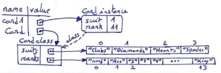
Alternatively, we can access a class variable via the object, for example:
>>> print(card1.suits[1]) Diamonds
What actually happens when accessing the variable suits on the object card1, is that Python will first try to find an instance variable with that name, and if that doesn't exist, following the link to the class of this instance look for a class variable with that name. This means that we could also have implemented the __str__ method above as follows (it will first look for a variable on the object itself, and if it doesn't find it there look in the class):
def __str__(self): return (self.ranks[self.rank] + " of " + self.suits[self.suit])
Personally, I prefer the former notation where it is also more explicit that we are actually accessing a class variable.
Unlike instance variables, which can have different values for each different instance of a same class, class attributes are shared by all instances of the same class. The advantage of this is that we can use any Card object to access the class attributes:
>>> card2 = Card(1, 3) >>> print(card2) 3 of Diamonds >>> print(card2.suits[1]) Diamonds
However, because every Card instance references the same class attribute, we have an aliasing situation. The disadvantage of that is that if we would modify a class attribute, this modification would affect every instance of that class. For example, if we decide that Jack of Diamonds should really be called Jack of Swirly Whales, we could do this:
>>> card1.suits[1] = "Swirly Whales" >>> print(card1) Jack of Swirly Whales
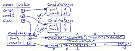
The problem is that all of the Diamonds just became Swirly Whales:
>>> print(card2) 3 of Swirly Whales
It is usually not a good idea to modify class attributes. If you do, be aware that the value will change for all instances of that class.
Comparing cards
For primitive types, there are six relational operators ( <, >, ==, <=, >=, !=) that compare values and determine when one is greater than, less than, or equal to another. If we want our own types to be comparable using the syntax of these relational operators, we need to define six corresponding magic methods in our class.
We'd like to start with a single method named cmp that captures the logic of ordering. By convention, a comparison method takes two parameters, self and other, and returns 1 if the first object is greater, -1 if the second object is greater, and 0 if they are equal to each other.
Some types are completely ordered, which means that we can compare any two elements and tell which is bigger. For example, the integers and the floating-point numbers are completely ordered. Some types are unordered, which means that there is no meaningful way to say that one element is bigger than another. For example, the fruits are unordered, which is why we cannot compare apples and oranges, and we cannot meaningfully order a collection of images, or a collection of cellphones.
Playing cards are partially ordered, which means that sometimes we can compare cards and sometimes not. For example, we know that the 3 of Clubs is higher than the 2 of Clubs, and the 3 of Diamonds is higher than the 3 of Clubs. But which is better, the 3 of Clubs or the 2 of Diamonds? One has a higher rank, but the other has a higher suit.
In order to make cards comparable, we have to decide which is more important, rank or suit. To be honest, the choice is arbitrary. For the sake of choosing, we will say that suit is more important, because a new deck of cards comes sorted with all the Clubs together, followed by all the Diamonds, and so on.
With that decided, we can write cmp:
def cmp(self, other): # Check the suits if self.suit > other.suit: return 1 if self.suit < other.suit: return -1 # Suits are the same... check ranks if self.rank > other.rank: return 1 if self.rank < other.rank: return -1 # Ranks are the same... it's a tie return 0
Note that in this ordering, Aces (1) appear lower than Deuces (2).
Now, we can define the six magic methods that do the overloading of each of the relational operators for us:
def __eq__(self, other): # equality return self.cmp(other) == 0 def __le__(self, other): # less than or equal return self.cmp(other) <= 0 def __ge__(self, other): # greater than or equal return self.cmp(other) >= 0 def __gt__(self, other): # strictly greater than return self.cmp(other) > 0 def __lt__(self, other): # strictly less than return self.cmp(other) < 0 def __ne__(self, other): # not equal return self.cmp(other) != 0
With this machinery in place, the relational operators now work as we'd like them to:
>>> card1 = Card(1, 11) >>> card2 = Card(1, 3) >>> card3 = Card(1, 11) >>> card1 < card2 False >>> card1 == card3 True
Decks
Now that we have objects to represent Cards, the next logical step is to define a class to represent a Deck. Of course, a deck is made up of cards, so each Deck object will contain a list of cards as an attribute. Some card games will need at least two different decks --- a red deck and a blue deck.

The following is a class definition for the Deck class. The initialisation method creates the attribute cards and generates the standard pack of fifty-two cards:
class Deck: def __init__(self): self.cards = [] for suit in range(4): for rank in range(1, 14): self.cards.append(Card(suit, rank))
The easiest way to populate the deck is with a nested loop. The outer loop enumerates the suits from 0 to 3. The inner loop enumerates the ranks from 1 to 13. (Remember that range(m, n) generates integers from m up to, but not including, n.) Since the outer loop iterates four times, and the inner loop iterates thirteen times, the total number of times the body is executed is 52 (13 * 4). Each iteration creates a new instance of Card with the current suit and rank, and appends that card to the cards list. (Remember that whenever the Card constructor method is invoked a new instance of class Card is created.)
With this in place, we can instantiate some decks:
red_deck = Deck() blue_deck = Deck()
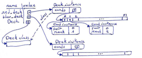
Printing the deck
As usual, when we define a new type we would like a way to print the contents of a Deck instance. One way to do so would be to implement a method to traverse the list of cards in the deck and print each Card:
class Deck: ... def print_deck(self): for card in self.cards: print(card)
Here, and from now on, the ellipsis (...) indicates that we have omitted the other methods in the class.
>>> red_deck.print_deck()
However, as we don't like chatterbox methods that call print, a better alternative to print_deck would be to write a string conversion method __str__ for the Deck class. The advantage of __str__ is that it is more flexible. Rather than just printing the contents of the object, it generates a string representation that other parts of the program can manipulate before printing, or store for later use. Here is a version of __str__ that returns a string representation of a Deck. To add a bit of flair to it, it arranges the cards in a cascade where each card is indented one space more than the previous card:
class Deck: ... def __str__(self): s,spaces = "","" for c in self.cards: s = s + spaces + str(c) + "\n" spaces += " " return s
This example demonstrates several features. First, instead of looping over the range of all cards, using an expression like for i in range(len(self.cards)), and to access each card using its index i, as in self.cards[i], instead we simply traverse self.cards and assign each card to a variable c.
Second, instead of using the print command to print the cards, we use the str function to get their print representation. Passing an object as an argument to str, i.e. str(c), is equivalent to invoking the __str__ method on the object, i.e. c.__str__() .
Thirdly, we are using the variables s and spaces as accumulators. Initially, s and spaces are empty strings. Each time through the loop, a new string is generated and concatenated to the old value of s to get the new value. Similarly, each time through the loop a single space is added to spaces to increase the indentation level. When the loop ends, s finally contains the complete string representation of the Deck, which looks like this:
>>> red_deck = Deck() >>> print(red_deck) Ace of Clubs 2 of Clubs 3 of Clubs 4 of Clubs 5 of Clubs 6 of Clubs 7 of Clubs 8 of Clubs 9 of Clubs 10 of Clubs Jack of Clubs Queen of Clubs King of Clubs Ace of Diamonds 2 of Diamonds ...
And so on. Even though the result appears on 52 lines, it is one long string that contains newlines.
Shuffling the deck
If a deck is perfectly shuffled, then any card is equally likely to appear anywhere in the deck, and any location in the deck is equally likely to contain any card.
To shuffle the deck, we will use the randrange function from the random module. With two integer arguments, a and b, randrange chooses a random integer in the range a <= x < b. Since the upper bound is strictly less than b, we can use the length of a list as the second parameter, and we are guaranteed to get a legal index in the list of cards. For example, if rng has already been instantiated as a random number source, this expression chooses the index of a random card in a deck:
rng.randrange(0, len(self.cards))
An easy way to shuffle the deck is by traversing the cards and swapping each card with a randomly chosen one. It is possible that the card will be swapped with itself, but that is fine. In fact, if we precluded that possibility, the order of the cards would be less than entirely random:
class Deck: ... def shuffle(self): import random rng = random.Random() # Create a random generator num_cards = len(self.cards) for i in range(num_cards): j = rng.randrange(i, num_cards) (self.cards[i], self.cards[j]) = (self.cards[j], self.cards[i])
>>> red_deck.shuffle() >>> print(red_deck)
Rather than assuming that there are fifty-two cards in the deck, we get the actual length of the list and store it in num_cards. This avoids having hardcoded numbers in the code, so that the algorithm is more generic and can be reused easily for other sizes of decks (such as those used for the blackjack card game).
Secondly, rather than looping over all cards, we now use a loop variable i to loop over the range of all cards, and access each card using its index i. We swap the current card at index i with one at a higher index j, chosen randomly from the cards that haven't been shuffled yet. Then we swap the current card (i) with the selected card (j) using a tuple assignment:
(self.cards[i], self.cards[j]) = (self.cards[j], self.cards[i])
While this is a good shuffling method, a random number generator object also has a shuffle method that can shuffle elements in a list, in place. So we could rewrite this function to use the one provided for us:
class Deck: ... def shuffle(self): import random rng = random.Random() # Create a random generator rng.shuffle(self.cards) # Use its shuffle method
Removing and dealing cards
Another method that would be useful for the Deck class is remove, which takes a card as a parameter, removes it and returns True, or False if the card was not in the deck (for example because it already has been removed before):
class Deck: ... def remove(self, card): if card in self.cards: self.cards.remove(card) return True else: return False
The in operator returns True if the first operand is in the second. If the first operand is an object, Python uses the object's __eq__ method to determine equality with items in the list. Since the __eq__ we provided in the Card class checks for deep equality, the remove method checks for deep equality.
To deal cards, we want to remove and return the top card. The list method pop provides a convenient way to do that:
class Deck: ... def pop(self): return self.cards.pop()
Actually, pop removes the last card in the list, so we are actually dealing from the bottom of the deck.
One more operation that we are likely to want is the Boolean function is_empty, which returns True if the deck contains no more cards:
class Deck: ... def is_empty(self): return self.cards == []
Glossary
- accumulator
- A variable used in a loop to accumulate a series of values, such as by concatenating them onto a string or adding them to a running sum.
- class attribute
- A variable that is defined inside a class definition but outside any method. Class attributes are accessible from any method in the class and are shared by all instances of the class.
- class variable
- synonym for class attribute
- encode
- To represent one type of value using another type of value by constructing a mapping between them.
- magic methods for relational operators
__eq__ (equals) overloads the == operator
__le__ (equals) overloads the <= operator
__ge__ (equals) overloads the >= operator
__lt__ (equals) overloads the < operator
__gt__ (equals) overloads the > operator
__ne__ (equals) overloads the != operator
References
| [ThinkCS] | How To Think Like a Computer Scientist --- Learning with Python 3 |
Inheritance
Source: this section is heavily based on Chapter 23 of [ThinkCS] though adapted to better fit with the contents, terminology and notations of this particular course.
Inheritance
The language feature most often associated with object-oriented programming is inheritance. Inheritance is the ability to define a new class that is a modified version of an existing class.
The primary advantage of this feature is that you can add new methods to a class without modifying the existing class. It is called inheritance because the new class inherits all of the methods of the existing class. Extending this metaphor, the existing class is sometimes called the parent class. The new class is called the child class or sometimes subclass.
Inheritance is a powerful feature. Some programs that would be complicated without inheritance can be written concisely and simply with it. Also, inheritance facilitates code reuse, since you can customise the behaviour of parent classes without having to modify them. In some cases, the inheritance structure reflects the natural structure of a problem, which makes the program easier to understand.
On the other hand, inheritance can sometimes make programs difficult to read. When a method is invoked, it is sometimes not clear where to find its definition, since the relevant code may be scattered among several classes. If the natural structure of a problem does not lend itself to inheritance, sometimes a more elegant solution without using inheritance is more appropriate. In general, as a computer scientist it is good to know a few different programming paradigms so that you can always choose the one that is most suited for the problem at hand.
In this chapter we will demonstrate the use of inheritance as part of a program that plays the card game [OldMaid]. One of our goals is to write the program in such a way that parts of its code could easily be reused to implement other card games. Furthermore, to implement the card game we will build upon the Card and Deck classes which we already introduced in the previous chapter.
A hand of cards
For almost any card game, we need to represent a hand of cards, i.e. the set of cards a player is holding in his hand. A Hand is similar to a Deck. Both are made up of a set of cards, and both require operations like adding and removing cards. Also, we might like the ability to shuffle both decks and hands.
But a Hand is also different from a Deck in certain ways. Depending on the game being played, we might want to perform some operations on hands that don't make sense for a deck. For example, in poker we might classify a hand (straight, flush, etc.) or compare it with another hand. In bridge, we might want to compute a score for a hand in order to make a bid.
This situation suggests the use of inheritance. If Hand is a subclass of Deck, it will have all the methods of Deck, but new methods can be added.
We add the code in this chapter to our Cards.py file from the previous chapter. In the class definition, the name of the parent class appears in parentheses:
class Hand(Deck): pass
This statement indicates that the new Hand class inherits from the existing Deck class. Such an empty child class would provide exactly the same behaviour as its super class. (In other words, instances of the child class understand exactly the same methods as instances of the super class.) This is not very useful, unless we add a few additional methods and instance variables.
We start by adding a constructor that initialises the attributes for a Hand, which are name and cards. The string name identifies this hand, probably by the name of the player that holds it. The name is an optional parameter with the empty string as default value. cards is the list of cards in the hand, initialised to the empty list:
class Hand(Deck): def __init__(self, name=""): self.cards = [] self.name = name
For just about any card game, it is necessary to add and remove cards from a hand. Removing cards is already taken care of, since Hand inherits remove from Deck. (In other words, since the super or parent class Deck already implements the method remove, any instance of class Hand will automatically understand that method as well.) But we still have to implement an add method:
class Hand(Deck): ... def add(self, card): self.cards.append(card)
Again, the ellipsis ... indicates that we have omitted other methods. The list append method adds the new card to the end of the list of cards held in the hand.
Dealing cards
Now that we have a Hand class, we want to deal cards from the Deck into hands. It is not immediately obvious whether this method should go in the Hand class or in the Deck class, but since it operates on a single deck and (possibly) several hands, it is more natural to put it in Deck.
deal should be fairly general, since different games will have different requirements. We may want to deal out the entire deck at once or add one card to each hand.
deal takes two parameters, a list (or tuple) of hands and the total number of cards to deal. If there are not enough cards in the deck, the method deals out all of the cards and stops:
class Deck: ... def deal(self, hands, num_cards=None): if num_cards==None : # if no value given for how many cards num_cards = len(self.cards) # to deal then deal all cards in deck num_hands = len(hands) for i in range(num_cards): if self.is_empty(): break # Break if out of cards card = self.pop() # Take the top card hand = hands[i % num_hands] # Whose turn is next? hand.add(card) # Add the card to the hand
The second parameter, num_cards, is optional; if no value is given for how many cards to deal, then we set the value to the size of the deck, so that all of the cards in the deck will get dealt.
The loop variable i goes from 0 to num_cards-1. Each time through the loop, a card is removed from the deck using the list method pop, which removes and returns the last item in the list.
The modulus operator (%) allows us to deal cards in a round robin (one card at a time to each hand). When i is equal to the number of hands in the list, the expression i % num_hands wraps around to the beginning of the list (index 0).
Printing a Hand
To print the contents of a hand, we can take advantage of the __str__ method inherited from Deck. For example:
>>> deck = Deck() >>> deck.shuffle() >>> hand = Hand("frank") >>> deck.deal([hand], 5) >>> print(hand) 2 of Spades 3 of Spades 4 of Spades Ace of Hearts 9 of Clubs
Although it is convenient to inherit the existing method, there is additional information in a Hand object we might want to include when we print one. To do that, we can provide a __str__ method in the Hand class that overrides the one in the Deck class:
class Hand(Deck) ... def __str__(self): s = "Hand " + self.name if self.is_empty(): s += " is empty\n" return s else: s += " contains\n" return s + Deck.__str__(self)
Initially, s is a string that identifies the hand. If the hand is empty, the program appends the words is empty and returns s.
Otherwise, the program appends the word contains and the string representation of the Deck, computed by invoking the __str__ method in the Deck class on self.
>>> deck = Deck() >>> deck.shuffle() >>> hand = Hand("frank") >>> deck.deal([hand], 5) >>> print(hand) Hand frank contains 2 of Spades 3 of Spades 4 of Spades Ace of Hearts 9 of Clubs
Method overriding and super calls
Let us analyse the previous string conversion method a bit more closely. Something very interesting is going on there! The method __str__ of the Hand class is said to override the one of the Deck class.
The word override has a very specific meaning here. It is not synonymous with the word overwrite. We do more than simply overwriting the parent class' implementation of __str__ by replacing it with a new one. In fact, the new implementation refines the old one, by making use of it, and doing a bit more. This combination of overwriting a method of the parent class, while at the same time refining it in such a way that the new implementation makes use of the old one, is called method overriding.
In the code above this happens in the expression Deck.__str__(self) inside the implementation of the method __str__(self) of the Hand class. This is an example of an explicit super call. The Hand's method __str__(self) calls __str__(self) on the super class Deck by explicitly referring to that super class.
Note that in the expression Deck.__str__(self), it may seem odd to pass self, which refers to the current Hand, to a Deck method, until you remember that a Hand is a kind of Deck. Hand objects can do everything Deck objects can, so it is legal to pass a Hand to a Deck method.
In general, it is always legal to use an instance of a subclass in place of an instance of a parent class.
An alternative way to write the __str__ method in the Hand class would be to make use of the special super() method in Python:
class Hand(Deck) ... def __str__(self): s = "Hand " + self.name if self.is_empty(): s += " is empty\n" return s else: s += " contains\n" return s + super().__str__()
The only change with respect to the previous implementation is the last line. Rather than referring to the super class Deck explicitly, the super() method allows us to refer to that super class implicitly. Also note that we don't have to pass self as an argument anymore when making such a super call.
The main advantage of using super() is that it allows us to avoid referring to the super class explicitly by name. This is considered as good object-oriented programming style. Most other object-oriented programming languages have a similar super keyword to allow methods overriding a method in their parent class, to call and extend that parent method.
The CardGame class
The CardGame class takes care of some basic chores common to all games, such as creating the deck and shuffling it:
class CardGame: def __init__(self): self.deck = Deck() self.deck.shuffle()
This is the first case we have seen where the initialisation method performs a significant computation, beyond initialising attributes. For more complex classes, like this one, that will often be the case. (As a side note, the initialisation method of a subclass will also often refine the initialisation method of its parent class using a super call. That is not the case here since CardGame is not a subclass.)
To implement specific games, we can inherit from CardGame and add features for the new game. As an example, we'll write a simulation for the [OldMaid] card game.
The object of Old Maid is to get rid, as soon as possible, of all the cards in your hand. You do this by matching cards by rank and colour. For example, the 4 of Clubs ♣︎ matches the 4 of Spades ♠︎ since they have the same rank (4) and both suits (♣︎,♠︎) are black. The Jack of Hearts ♥︎ matches the Jack of Diamonds ♦︎ since both Jacks are of the red colour.
Before starting the game, the Queen of Clubs is removed from the deck. (Other variants of the [OldMaid] game exist where the card removed from the deck is another one, but that doesn't change the essence of the game.) As a consequence of having removed the Queen of Clubs, its corresponding card, the Queen of Spades, will never be matched during the game. The player who remains with this card, the old maid, at the end of the game, loses the game.
The 51 remaining cards are now dealt to the players in a round robin fashion. After the deal, all players can discard all matching pairs of cards they have in their hand.
When no more matches can be made, the actual play begins. In turn, each player picks a card (without looking) from his closest neighbor to the left who still has cards. If the chosen card matches a card in the player's own hand, he can discard this pair from his hand. Otherwise, the chosen card is added to the player's hand. Eventually, as the game continues, all possible matches are made, except for the Queen of Spades (for which no match exists, as the Queen of Clubs was removed from the deck before starting the game). The player who remains with the Queen of Spades in his hand loses the game. (This game is particular in the sense that it has a unique loser, not a winner.)
In our computer simulation of the game, the computer will play all hands. Unfortunately, some funny nuances of the real game are lost. In a real game, the player with the Old Maid goes to some effort to get their closest neighbor to pick that card, by displaying it a little more prominently, or perhaps failing to display it more prominently, or even failing to fail to display that card more prominently. The computer simply picks a neighbor's card at random.
OldMaidHand class
A hand for playing the Old Maid game requires some abilities beyond the general abilities of a Hand, such as the ability to remove matching cards from the hand. We will therefore define a new class, OldMaidHand, that inherits from Hand to reuse its functionality, and provides an additional method called remove_matches:
class OldMaidHand(Hand): def remove_matches(self): count = 0 original_cards = self.cards.copy() for i in range(0,len(original_cards)): card = original_cards[i] for j in range(i+1,len(original_cards)): match = original_cards[j] if match == Card(3 - card.suit, card.rank): self.cards.remove(card) self.cards.remove(match) count += 1 print("Hand {0}: {1} matches {2}".format(self.name, card, match)) break return count
We start by making a copy of the list of cards, so that we can traverse the copy while removing cards from the original. Since self.cards will be modified in the loop, we don't want to use it to control the traversal. Python (or any other programming language, for that matter) can get quite confused if it is traversing a list that is changing while being traversed!
For each card in our hand (outer loop), we iterate over all the remaining cards in our hand (inner loop) to check whether they match that card. In the inner loop, we are smart and only consider cards after the current card being compared, since all the ones before have already been compared.
We have a match if the match has the same rank and the other suit of the same color. Conveniently, the expression 3 - card.suit turns a Club ♣︎ (suit 0) into a Spade ♠︎ (suit 3) and a Diamond ♦︎ (suit 1) into a Heart ♥︎ (suit 2). You should satisfy yourself that the opposite operations also work. This clever trick works because of how we encoded suits as numbers. A clever encoding often may make certain operations surprisingly easy.
Whenever we find a match, we remove both the card and its match from our hand, and jump out of the inner loop, since no other matches for this card will be found.
The following example demonstrates how to use remove_matches:
>>> game = CardGame() >>> hand = OldMaidHand("frank") >>> game.deck.deal([hand], 13) >>> print(hand) Hand frank contains 2 of Hearts 6 of Diamonds 9 of Clubs 6 of Hearts Jack of Diamonds 7 of Diamonds 10 of Spades 7 of Clubs 3 of Hearts 7 of Hearts 3 of Spades 10 of Clubs 8 of Clubs >>> count = hand.remove_matches() Hand frank: 6 of Diamonds matches 6 of Hearts Hand frank: 7 of Diamonds matches 7 of Hearts Hand frank: 10 of Spades matches 10 of Clubs >>> print("{} matches found".format(count)) 3 matches found >>> print(hand) Hand frank contains 2 of Hearts 9 of Clubs Jack of Diamonds 7 of Clubs 3 of Hearts 3 of Spades 8 of Clubs
Notice that there is no __init__ method for the OldMaidHand class. We inherit it from Hand.
Alternative implementation
Here's an alternative and slightly more compact implementation of the remove_matches method. Which one you prefer is a matter of personal taste.
class OldMaidHand(Hand): def remove_matches(self): count = 0 original_cards = self.cards.copy() for card in original_cards: match = Card(3 - card.suit, card.rank) if match in self.cards: self.cards.remove(card) self.cards.remove(match) count += 1 print("Hand {0}: {1} matches {2}".format(self.name, card, match)) return count
OldMaidGame class
Now we can turn our attention to the game itself. OldMaidGame is a subclass of CardGame. Since __init__ is inherited from CardGame, a new OldMaidGame object already contains a new shuffled deck. OldMaidGame defines a new method called play that takes a list of player names as a parameter. Calling this play method launches the game:
OldMaidGame().play(["kim","charles","siegfried"])
The play method is defined as follows:
class OldMaidGame(CardGame): ... def play(self, names): # Remove Queen of Clubs queen_clubs = Card(0,12) self.deck.remove(queen_clubs) # Make a hand for each player self.hands = [] for name in names: self.hands.append(OldMaidHand(name)) # Deal the cards self.deck.deal(self.hands) print("---------- Cards have been dealt") self.print_hands() # Remove initial matches print("---------- Discarding matches from hands") matches = self.remove_all_matches() print("---------- Matches have been discarded") self.print_hands() # Play until all 50 cards are matched # in other words, until 25 pairs have been matched print("---------- Play begins") turn = 0 num_players = len(names) while matches < 25: matches += self.play_one_turn(turn) turn = (turn + 1) % num_players print("---------- Game is Over") self.print_hands()
Some of the steps of the game have been separated into methods. The auxiliary method print_hands is pretty straightforward:
class OldMaidGame(CardGame): ... def print_hands(self): for hand in self.hands: print(hand)
remove_all_matches traverses the list of hands and invokes remove_matches on each:
class OldMaidGame(CardGame): ... def remove_all_matches(self): count = 0 for hand in self.hands: count += hand.remove_matches() return count
count is an accumulator that adds up the number of matches in each hand. When we've gone through every hand, the total is returned (count). We need this count to stop the game after 25 matches have been found. Indeed, when the total number of matches reaches 25, we know that 50 cards have been removed from the hands, which means that only 1 card is left (the old maid) and the game is over.
The variable turn keeps track of which player's turn it is. It starts at 0 and increases by one each time; when it reaches num_players, the modulus operator wraps it back around to 0.
The method play_one_turn takes a parameter that indicates whose turn it is. The return value is the number of matches made during this turn:
class OldMaidGame(CardGame): ... def play_one_turn(self, i): print("Player" + str(i) + ":") if self.hands[i].is_empty(): return 0 neighbor = self.find_neighbor(i) picked_card = self.hands[neighbor].pop() self.hands[i].add(picked_card) print("Hand", self.hands[i].name, "picked", picked_card) count = self.hands[i].remove_matches() self.hands[i].shuffle() return count
If a player's hand is empty, that player is out of the game, so he or she does nothing and 0 matches are returned.
Otherwise, a turn consists of finding the first player on the left that has cards, taking one card from the neighbor, and checking for matches. Before returning, the cards in the hand are shuffled so that the next player's choice is random.
The method find_neighbor starts with the player to the immediate left and continues around the circle until it finds a player that still has cards:
class OldMaidGame(CardGame): ... def find_neighbor(self, i): num_hands = len(self.hands) for next in range(1,num_hands): neighbor = (i + next) % num_hands if not self.hands[neighbor].is_empty(): return neighbor
If find_neighbor ever went all the way around the circle without finding cards, it would return None and cause an error elsewhere in the program. Fortunately, we can prove that that will never happen (as long as the end of the game is detected correctly).
Putting it all together
In the appendix chapter you will find the full code of all classes we defined above, as well as a sample output of a run of the game.
Glossary
- ancestor class
- A parent class, or an ancestor of the parent class.
- child class
- A new class created by inheriting from an existing class; also called a subclass.
- inheritance
- The ability to define a new class that is a modified version of a previously defined class.
- method overriding
- When, in addition to overwriting a method higher up the hierarchy, the implementation of that new method also refines the old one, by making use of it through a super call, and doing a bit more.
- method overwriting
- When a method defined in a child class replaces the implementation of a method with the same name defined in a parent or ancestor class.
- parent class
- The class from which a child class inherits; also called a superclass
- subclass
- Another word for child class.
- superclass
- another word for parent class.
- super call
- A super call can be used to gain access to inherited methods – from a parent or ancestor class – that have been overridden in a child class. This can either be done by explicitly referring to that parent class, or implicitly by using the special super() function.
Linked lists
Source: this section is largely based on Chapter 24 of [ThinkCS] though adapted to better fit with the contents, terminology and notations of this particular course. In particular, some of the code in this chapter has been adapted to use a more object-oriented style.
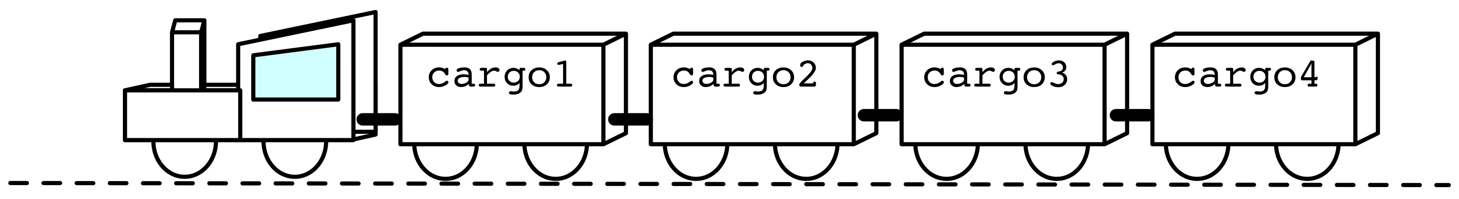
Embedded references
We have seen examples of attributes that refer to other objects. For example, the CardGame class referred to a Deck object as one of its attributes. We call such objects contained in another one embedded references.
We have also seen examples of data structures, such as lists and tuples. For example, Deck objects contain a list of Card objects.
A data structure is a mechanism for grouping and organising data to make it easier to use.
In this section, we will use object-oriented programming and objects with embedded references to define our own data structure, a data structure commonly known as a linked list.
Linked lists are made up of Node objects, where each node (the last node excepted) contains a reference to the next node in the linked list. In addition, each node carries a unit of data called its cargo.
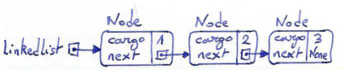
A linked list can be regarded as a recursive data structure because it has a recursive definition:
A linked list is either:
- the empty list, represented by None, or
- a node that contains a cargo object and a reference to a linked list.
Recursive data structures lend themselves to recursive methods. A recursive method is a method that invokes itself, typically on a subset of the data on which it was originally invoked. For example, a method to print a linked list could first print the cargo of the node at the head of the list, and then recursively invoke itself on the embedded linked list that node refers to.
The Node class
As always when writing a new class, we'll start with the initialisation and __str__ methods so that we can test the basic mechanism of creating and displaying the new type:
class Node: """ Represents a Node in a LinkedList data structure. """ def __init__(self, cargo=None, next=None): """ Creates a new Node object. @pre: - @post: A new Node object has been initialised. A node can contain a cargo and a reference to another node. If none of these are given, the node is initialised with empty cargo (None) and no reference (None). """ self.cargo = cargo self.next = next def __str__(self): """ @pre: - @post: Returns a print representation of the cargo contained in this Node. """ return str(self.cargo)
As usual, the parameters for the initialisation method are optional. By default, both the cargo and the link to the next node, are set to None.
The string representation of a node is just the string representation of its cargo. Since any value can be passed to the str function, we can store any value in a linked list.
To test the implementation so far, we can create a Node object and print it:
>>> node = Node("test") >>> print(node) test
To make it more interesting, we will now try to create a linked list with three nodes. First we create each of the three nodes.
>>> node1 = Node(1) >>> node2 = Node(2) >>> node3 = Node(3)
This code creates three nodes, but we don't have a linked list yet because the nodes are not linked. The memory diagram looks like this:
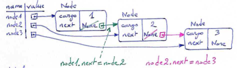
To link the nodes, we have to make the first node refer to the second one and the second one to the third:
>>> node1.next = node2 >>> node2.next = node3 >>> linkedlist = node1
The next reference of the third node remains None, which indicates that it is the end of the linked list. Now the memory diagram looks like this:
Now you know how to create nodes and link them into lists. What might be less clear at this point is why.
Linked lists as collections
Linked lists and other data structures are useful because they provide a way to assemble multiple objects into a single entity, sometimes called a collection. In our example, the first node of a linked list serves as a reference to the entire list (since from the first node, all the other nodes in the list can be reached).
To pass a linked list as a parameter, we only have to pass a reference to its first node. For example, the function print_list below takes a single node as an argument. Starting with the head of a linked list, it prints each node until it gets to the end:
def print_list(node): """ Prints the cargo of this node and of each node it is linked to. @pre: node is an instance of class Node @post: Has printed a space-separated list of the form "a b c ... ", where "a" is the string-representation of this node, "b" is the string-representation of my next node, and so on. A space is printed after each printed value. """ while node is not None: print(node, end=" ") node = node.next
To invoke this function, we pass a reference to the first node:
>>> print_list(node1) 1 2 3
Inside print_list we have a reference to the first node of the linked list. From there, to get to the next nodes, we can use the next attribute of each node. To traverse a linked list, it is common to use a loop variable like node to refer to each of the nodes in succession. This diagram shows the different values that the node variable takes on:
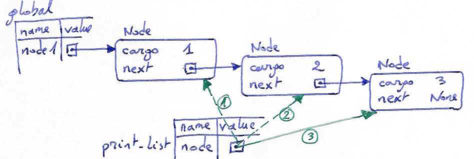
Linked lists and recursion
Since the linked list data structure is defined as a class, it would have been more natural to define the print_list function as a method on the Node class. When doing so, the method needs to be defined in a recursive way, by first printing the cargo of its head and then recursively invoking the print_list method on the next node, until no more nodes are left:
class Node: ... def print_list(self): """ Prints the cargo of this node and then recursively of each node connected to this one. @pre: The linked data structure of which this node is the head contains no loops. @post: Has printed a space-separated list of the form "a b c ... ", where "a" is the string-representation of this node, "b" is the string-representation of my next node, and so on. A space is printed after each printed value. """ print(self, end=" ") # print my head tail = self.next # go to my next node if tail is not None : # as long as the end of the list was not reached tail.print_list() # recursively print remainder of the list
To call this method, we just send it to the first node:
>>> node1.print_list() 1 2 3
In general, it is natural to express many operations on linked lists as recursive methods. The following is a recursive algorithm for printing a list backwards:
- Separate the list into two pieces: its first node (called the head); and the remainder (called the tail).
- Print the tail backward.
- Print the head.
The code which implements this algorithm looks surprisingly similar to the code of the print_list method above, the only difference being that now the head is printed after the recursive call, instead of before :
class Node: ... def print_backward(self): """ Recursively prints the cargo of each node connected to this node (in opposite order), then prints the cargo of this node as last value. @pre: The linked data structure of which this node is the head contains no loops. @post: Has printed a space-separated list of the form "... c b a", where a is my cargo (self), b is the cargo of the next node, and so on. The nodes are printed in opposite order: the last node's value is printed first. """ tail = self.next # go to my next node if tail is not None : # as long as end of list was reached tail.print_backward() # recursively print remainder backwards print(self, end = " ") # print my head
As before, to call this method, we just send it to the first node:
>>> node1.print_backward() 3 2 1
Can we prove that print_backward will always terminate? In fact, the answer is no: some (ill-formed) linked lists can make this method crash.
Infinite lists
There is nothing to prevent a node from referring back to an earlier node in the list, including itself. For example, this figure shows a list with two nodes, one of which refers to itself:
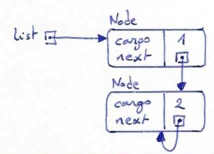
We could create such an infinite list as follows:
>>> node1 = Node(1) >>> node2 = Node(2) >>> node1.next = node2 >>> node2.next = node2
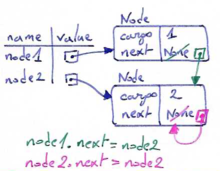
If we call either print_list or print_backward on this list, it will try to recurse infinitely, which soon leads to an error like:
RecursionError: maximum recursion depth exceeded
This sort of behaviour makes infinite lists difficult to work with. Nevertheless, they are occasionally useful. For example, we might represent a number as a list of digits and use an infinite list to represent a repeating fraction.
Regardless, it is problematic that we cannot prove that print_list and print_backward terminate. The best we can do is the hypothetical statement, "if the list contains no loops, then these methods will terminate", and use this as a precondition to be satisfied by the methods.
Ambiguity between lists and nodes
When looking at the code of the print_list or print_backward methods above, there is sometimes ambiguity between whether a reference to a node should be interpreted as a reference to a single node or rather as a reference to an entire linked list having that node as its first node.
For example, when we write print(self, end=" ") we seem to regard self as referring to a single node that is the head of this linked list, and we use the print function to print the value of its cargo.
On the other hand, when assigning self.next to a variable named tail, we seem to be regarding self.next not as a single node but rather as the entire linked list that has the next node as first node.
The fundamental ambiguity theorem describes the ambiguity that is inherent in a reference to a node of a linked list: A variable that refers to a node of a linked list might treat the node as a single object or as the first in a list of nodes.
Modifying lists
There are two ways to modify a linked list. Obviously, we can change the cargo of one of its nodes, but the more interesting operations are the ones that add, remove, or reorder nodes.
As an example, let's write a method that removes the second node in the list and returns a reference to the removed node:
class Node: ... def remove_second(self): """ @pre: The linked data structure of which this node is the first node contains no loops. @post: Does nothing if the linked list with this node as head has no second node; else removes the second node from this linked list, and returns a reference to the removed and unlinked second node. """ first = self second = self.next # do nothing if there is no second node if second is None: return # Make the first node refer to the third first.next = second.next # Separate the second node from the rest of the list second.next = None return second
We are using temporary variables first and second here to make the code more readable. Here is how to use this method:
>>> node1.print_list() 1 2 3 >>> removed = node1.remove_second() >>> removed.print_list() 2 >>> node1.print_list() 1 3
This state diagram shows the effect of the operation:
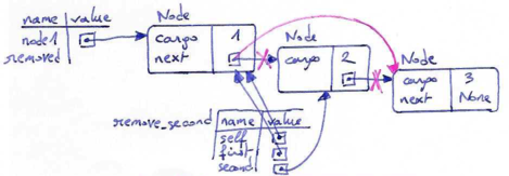
Wrappers and helpers
It is often useful to divide a list operation into two methods. For example, to print a list backward in a more conventional format [3 2 1], we can use the print_backward method to print 3 2 1 but we need a separate method to print the brackets. Let's call it print_backward_nicely:
class Node: ... def print_backward_nicely(self): """ @pre: The linked data structure of which this node is the head contains no loops. @post: Has printed a space-separated list of the form "[ ... c b a ]", where a is my cargo (self), b is the cargo of the next node, and so on. The nodes are printed in opposite order: the last node's value is printed first. A space is printed after and before the opening and closing bracket, as well as between any two elements. An empty linked is printed as "[ ]" """ print("[", end=" ") self.print_backward() print("]")
When we use this method elsewhere in the program, we invoke print_backward_nicely directly, and it invokes print_backward on our behalf. In that sense, print_backward_nicely acts as a wrapper, and it uses print_backward as a helper.
The LinkedList class
There remains a subtle problem with the way we have been implementing linked lists so far, namely that the empty list is represented in a different way (None) as a non-empty list (a collection of Node objects chained to each other). To solve this problem, we will create a new class called LinkedList. Its attributes are an integer that contains the length of the list and a reference to the first node. In case of an empty list the length attribute is 0 and the reference to the first node is None. LinkedList objects serve as handles for manipulating lists of Node objects:
class LinkedList: """ Represents a linked list datastructure. """ def __init__(self): """ Initialises a new LinkedList object. @pre: - @post: A new empty LinkedList object has been initialised. It has 0 length, contains no nodes and its head points to None. """ self.length = 0 self.head = None
Adding an element to the front of a LinkedList object can be defined straightforwardly. The method add is a method for LinkedLists that takes an item of cargo as an argument and puts it in a newly created note at the head of the list. This works regardless of whether the list is initially empty or not.
class LinkedList: ... def add(self, cargo): """ Adds a new Node with given cargo to the front of this LinkedList. @pre: self is a (possibly empty) LinkedList. @post: A new Node object is created with the given cargo. This new Node is added to the front of the LinkedList. The length counter has been incremented. The head of the list now points to this new node. Nothing is returned. """ node = Node(cargo) node.next = self.head self.head = node self.length += 1
The LinkedList class also provides a natural place to put wrapper functions like our method print_backward_nicely, which we can make a method of the LinkedList class:
class LinkedList: ... def print_backward(self): """ Prints the contents of this LinkedList and its nodes, back to front. @pre: self is a (possibly empty) LinkedList @post: Has printed a space-separated list of the form "[ ... c b a ]", where "a", "b", "c", ... are the string representation of each of the LinkedList's nodes. The nodes are printed in opposite order: the last nodes' value are printed first. A space is printed after and before the opening and closing bracket, as well as between any two elements. An empty linked is printed as "[ ]" """ print("[", end=" ") if self.head is not None: self.head.print_backward() print("]")
We renamed print_backward_nicely to print_backward when defining it on the LinkedList class. This is a nice example of polymorphism. There are now two methods named print_backward: the original one defined on the Node class (the helper); and the new one on the LinkedList class (the wrapper). When the wrapper method invokes self.head.print_backward(), it is invoking the helper method, because self.head is a Node object. To avoid calling this helper method on an empty list (when self.head is None), we added a condition to check for that situation.
In a similar way we can define a print method on the LinkedList class, to print the entire list nicely with surrounding brackets. This method is implemented in a very similar way to the print_backward method, using the print_list method on the Node class as a helper method.
class LinkedList: ... def print(self): """ Prints the contents of this LinkedList and its nodes. @pre: self is a (possibly empty) LinkedList @post: Has printed a space-separated list of the form "[ a b c ... ]", where "a", "b", "c", ... are the string representation of each of the linked list's nodes. A space is printed after and before the opening and closing bracket, as well as between any two elements. An empty linked is printed as "[ ]" """ print("[", end=" ") if self.head is not None: self.head.print_list() print("]")
The code below illustrates how to create and print linked lists using this new LinkedList class.
>>> l = LinkedList() >>> print(l.length) 0 >>> l.print() [ ] >>> l.add(3) >>> l.add(2) >>> l.add(1) >>> l.print() [ 1 2 3 ] >>> l.print_backward() [ 3 2 1 ]
The full code of this LinkedList class and its corresponding Node class are provided in an appendix. As opposed to the code above, in this appendix we also hid the attributes and provided some accessor and mutator methods to access and modify these attributes.
Other useful methods can be added to this LinkedList class, such as a method to remove the first element of a list. We leave this as an exercise to the reader.
Invariants
Some lists are well formed; others are not. For example, if a list contains a loop, it will cause many of our methods to crash, so we might want to require that lists contain no loops. Another requirement is that the length value in the LinkedList object should be equal to the actual number of nodes in the list.
Requirements like these are called invariants because, ideally, they should be true of every object all the time. Specifying invariants for objects is a useful programming practice because it makes it easier to prove the correctness of code, check the integrity of data structures, and detect errors.
One thing that is sometimes confusing about invariants is that there are times when they are violated. For example, in the middle of add, after we have added the node but before we have incremented length, the invariant is violated. This kind of violation is acceptable; in fact, it is often impossible to modify an object without violating an invariant for at least a little while. Normally, we require that every method that violates an invariant must restore the invariant.
If there is any significant stretch of code in which the invariant is violated, it is important for the comments to make that clear, so that no operations are performed that depend on the invariant.
Glossary
- cargo
- An item of data contained in a node. (The data carried by the node.)
- collection
- A collection is a data structure that assembles multiple objects into a single entity.
- data structure
- A mechanism for grouping and organising data to make it easier to use.
- embedded reference
- A reference to another object stored in an attribute of an object.
- fundamental ambiguity theorem
- A reference to a list node can be treated as a single object or as the first in a list of nodes.
- helper
- A method that is not invoked directly by a caller but is used by another method to perform part of an operation. Also called auxiliary method.
- invariant
- An assertion that should be true of an object at all times (except perhaps while the object is being modified).
- link
- An embedded reference used to link one object to another.
- linked list
- A data structure that implements a collection of elements using a sequence of linked nodes.
- node
- An element of a linked list, usually implemented as an object that carries a unit of data (its cargo) and that contains an embedded reference (a link) to another object of the same type.
- precondition
- An assertion that must be true in order for a method to work correctly.
- recursive data structure
- A recursive data structure, such as a linked list, is a data structure that can be defined in terms of itself. For example, we can say that a linked list is either the empty list, or a node that carries a cargo and a link to a linked list, containing the remaining data.
- recursive method
- A recursive method is a method that invokes itself, typically on a subset of the data on which it was originally invoked.
- singleton
- A linked list with a single node.
- wrapper
- A method that acts as a middleman between a caller and a helper method, often making the method easier or less error-prone to invoke.
References
| [ThinkCS] | How To Think Like a Computer Scientist --- Learning with Python 3 |
Appendix - Code of phone example
PhoneNumber class
class PhoneNumber : def __init__(self,c,z,pr,po) : self.country = c self.zone = z self.prefix = pr self.postfix = po def call(self) : print("Calling number " + str(self)) def __str__(self): return "+" + self.country + "(0)" + self.zone \ + "/" + self.prefix + self.postfix
Creating and using PhoneNumber objects
>>> number_kim = PhoneNumber("32","10","4","79111") >>> print(number_kim) +32(0)10/479111 >>> number_kim = PhoneNumber("32","10","4","79111") >>> print(number_kim) +32(0)10/479111 >>> number_kim.call() Calling number +32(0)10/479111
NokiaPhone class
class NokiaPhone : def __init__(self,s,p,t,n) : self.marque = "Nokia" self.serie = s self.poids = p self.taille = t self.numero = n def print_type(self) : print(self.marque + " " + str(self.serie)) def print_specs(self) : self.print_type() print("Poids: " + str(self.poids) + " g") print("Taille: " + self.taille + " mm") def print(self) : self.print_specs() print(self.numero) def __eq__(self, other) : return (self.marque == other.marque) \ and (self.serie == other.serie) \ and (self.poids == other.poids) \ and (self.taille == other.taille) def __str__(self) : return self.marque + " " + str(self.serie) + "\n" \ + "Poids: " + str(self.poids) + " g" + "\n" \ + "Taille: " + self.taille + " mm" + "\n"
Creating and using NokiaPhone objects
>>> phone_kim = NokiaPhone(5110,170,"132x48x31",number_kim) >>> phone_kim.print() Nokia 5110 Poids: 170 g Taille: 132x48x31 mm +32(0)10/479111 >>> phone_kim.print_specs() Nokia 5110 Poids: 170 g Taille: 132x48x31 mm >>> phone_kim.print_type() Nokia 5110 >>> print(phone_kim) Nokia 5110 Poids: 170 g Taille: 132x48x31 mm
Attention : phone_kim.print() ≠ print(phone_kim) ! Pourquoi ?
>>> number_charles = PhoneNumber("32","10","4","79222") >>> nokia_charles = NokiaPhone(7.1,160,"150x71x8",number_charles) >>> print(nokia_charles) Nokia 7.1 Poids: 160 g Taille: 150x71x8 mm >>> number_siegfried = PhoneNumber("32","10","4","79333") >>> nokia_siegfried = NokiaPhone(5110,170,"132x48x31",number_siegfried) >>> nokia_siegfried.print_specs() Nokia 5110 Poids: 170 g Taille: 132x48x31 mm >>> phone_charles = phone_kim >>> phone_charles.marque = "Alcatel" >>> phone_charles = None >>> print(phone_kim) Alcatel 5110 Poids: 170 g Taille: 132x48x31 mm >>> nokia_kim = NokiaPhone(5110,170,"132x48x31",number_kim) >>> nokia_siegfried = NokiaPhone(5110,170,"132x48x31",number_siegfried) >>> print(nokia_kim == nokia_siegfried) # appelera la méthode magique __eq__ True >>> print(nokia_kim is nokia_siegfried) # appelera la méthode magique __eq__ False >>> import copy >>> nokia_siegfried = copy.copy(nokia_kim) >>> nokia_kim.poids = 200 >>> print(nokia_kim) Nokia 5110 Poids: 200 g Taille: 132x48x31 mm >>> print(nokia_siegfried) Nokia 5110 Poids: 170 g Taille: 132x48x31 mm >>> kim_phone = NokiaPhone(5110,170,"132x48x31",number_kim) >>> siegfried_phone = copy.copy(kim_phone) >>> charles_phone = copy.deepcopy(kim_phone) >>> number_kim.postfix = "79000" >>> kim_phone.print() Nokia 5110 Poids: 170 g Taille: 132x48x31 mm +32(0)10/479000 >>> siegfried_phone.print() Nokia 5110 Poids: 170 g Taille: 132x48x31 mm +32(0)10/479000 >>> charles_phone.print() Nokia 5110 Poids: 170 g Taille: 132x48x31 mm +32(0)10/479111
Attention : le numéro de téléphone de Charles n'a pas changé (deep copy) mais le numéro de Siegried a changé (shallow copy).
Appendix - Worked out example: accounts
Classes and objects
First let us create a class representing bank accounts ("comptes en banque"):
class Compte : def __init__(self, titulaire) : self.titulaire = titulaire self.solde = 0
Now let us create an object of this class, representing someone's bank account:
>>> a = Compte("kim") >>> print(a.titulaire) kim >>> print(a.solde) 0 >>> a.solde = 10 >>> print(a.solde) 10 >>> a.solde += 1000 >>> print(a.solde) 1010
Hiding instance variables
Of course, we don't like it too much that our bank account details are so easily accessible from the outside. So let us try to hide the attributes:
class Compte : def __init__(self, titulaire) : self.__titulaire = titulaire self.__solde = 0
As you can see, you cannot easily access the instance attributes of an object of this class, such as an account's balance, anymore:
>>> a = Compte("kim") >>> a.__titulaire AttributeError: 'Compte' object has no attribute 'titulaire' >>> a.__solde AttributeError: 'Compte' object has no attribute '__solde'
Accessor methods
But oh, wait a minute, we need to be able to at least get access to it from the inside, so we need accessor methods that allow us to access these values, and while we are at it let's add a method to be able to print the account too:
class Compte : # initialiser def __init__(self, titulaire): self.__titulaire = titulaire self.__solde = 0 # accessor def titulaire(self): return self.__titulaire # accessor def solde(self): return self.__solde # print representation def __str__(self) : return "Compte de {} : solde = {}".format(self.titulaire(),self.solde())
Remember that when we define a method we write def solde(self): and shouldn't forget the self parameter. But when we call a method on self (or on another object) we write `self.solde() without the self-parameter and Python will implicitly bind the self-parameter to the receiver object.
If you don't know or don't remember how the format() method works on strings, look it up, it's not so crucial for this example; we could easily have written the __str__ method without it, but it leads to more compact code.
Also note how we use the accessors methods titulaire() and solde() in the __str__ method as well. This makes it easier to change the internal variable if we want to.
>>> a = Compte("kim") >>> print(a) Compte de kim : solde = 0 >>> print(a.titulaire()) kim
Mutator methods
Objects carry their own state and can provide their own methods to manipulate that state. We will now add two such mutator methods (they are called like that since they mutate the state of the object); one for redrawing money from the account, and another to deposit money on the account:
class Compte : # initialiser def __init__(self, titulaire): self.__titulaire = titulaire self.__solde = 0 # accessor def titulaire(self): return self.__titulaire # accessor def solde(self): return self.__solde # string representation def __str__(self) : return "Compte de {} : solde = {}".format(self.titulaire(),self.solde()) # *** No modifications above! Only the methods below were added... *** # mutator def deposer(self, somme): self.__solde += somme return self.solde() # mutator def retirer(self, somme): if self.solde() >= somme : self.__solde -= somme return self.solde() else : return "Solde insuffisant"
Now we can add or remove money from an account with the newly added methods:
>>> compte_charles = Compte("Charles") >>> print(compte_charles) Compte de Charles : solde = 0 >>> print(compte_charles.deposer(100)) 100 >>> print(compte_charles.retirer(90)) 10 >>> print(compte_charles.retirer(50)) Solde insuffisant >>> print(compte_charles.titulaire()) Charles
Class variables
While an object's instance variables carry the state of the object that is specific to each particular instance, sometimes it is also useful to have a state that is shared by all the objects of a same class. For example, all account objects may share the same interest rate. Such shared state common to all instances of a same class can be declared in a class variable, or class attribute, defined within the class:
class Compte : # class variable taux_interet = 0.02 def __init__(self, titulaire): self.__titulaire = titulaire self.__solde = 0 def titulaire(self): return self.__titulaire def solde(self): return self.__solde # We also modify the print representation to show the interest rate def __str__(self) : return "Compte de {0} : solde = {1:4.2f} \ntaux d'intérêt = {2}".format(self.titulaire(),self.solde(),self.taux_interet) def deposer(self, somme): self.__solde += somme return self.solde() def retirer(self, somme): if self.solde() >= somme : self.__solde -= somme return self.solde() else : return "Solde insuffisant"
Two different instances of this class share the same value for the class variable, but their instance variables may vary:
>>> compte_kim = Compte("Kim") >>> print(compte_kim) Compte de Kim : solde = 0.00 taux d'intérêt = 0.02 >>> compte_siegfried = Compte("Siegfried") >>> print(compte_siegfried) Compte de Siegfried : solde = 0.00 taux d'intérêt = 0.02
Changing the state of the class variable changes it for all instances of that class:
>>> Compte.taux_interet = 0.04 >>> print(compte_kim) Compte de Kim : solde = 0.00 taux d'intérêt = 0.04 >>> print(compte_siegfried) Compte de Siegfried : solde = 0.00 taux d'intérêt = 0.04
Shadowing
Attention! It is possible for an instance variable to have the same name as a class variable. Here, we add a new instance variable to an object that will shadow the value of the class variable.
>>> compte_kim.taux_interet = 0.03
Asking the object for that variable will now return the value of the newly assigned instance variable:
>>> print(compte_kim.taux_interet) 0.03
Even though the class variable still exists with its old value: newly assigned instance variable:
>>> print(Compte.taux_interet) 0.04
Asking other objects of this class for the value of that variable will still return the value of that class variable (in these other objects, the class variable wasn't shadowed by an instance variable.
>>> print(compte_siegfried.taux_interet) 0.04
Hiding class variables and class methods
Now that we have seen how to create a class variable, we can ask ourselves the question whether there is also a way to hide a class variable so that we cannot change it from the outside?
The answer is yes: add an __ to the name, just like we did with the instance variables. But then we also need to add an accessor and a mutator method if we want to read or write the class variable externally.
These need to be declared as class methods. Class methods are methods that should be invoked on the class, not on the instance.
class Compte : __taux_interet = 0.02 @classmethod def taux_interet(cls): return cls.__taux_interet @classmethod def set_taux_interet(cls,nouveau_taux): cls.__taux_interet = nouveau_taux def __init__(self, titulaire): self.__titulaire = titulaire self.__solde = 0 def titulaire(self): return self.__titulaire def solde(self): return self.__solde def __str__(self) : return "Compte de {0} : solde = {1:4.2f} \ntaux d'intérêt = {2}".format(self.titulaire(),self.solde(),self.taux_interet()) def deposer(self, somme): self.__solde += somme return self.solde() def retirer(self, somme): if self.solde() >= somme : self.__solde -= somme return self.solde() else : return "Solde insuffisant"
Note how the class methods take an extra parameter which, by convention, is named cls and that refers to the class, just like normal instance methods took an extra parameter self that refer to the receiving object.
>>> compte_kim = Compte("Kim") >>> Compte.taux_interet() 0.02
Note that, in Python, you can invoke the class method on the instance too! That may be a bit confusing, but what happens is that Python first tries to send the method to the object instance, and if it cannot find an instance method with that name it will invoke it instead as a class method on the class of that instance.
>>> compte_kim.taux_interet() 0.02
Inheritance
Now let us consider a special kind of account, a checkings account, which inherits from the general account type and adds one additional method.
Inheritance is one of the core concepts of object-oriented programming. It enables the creation of a new (refined) class from an existing one, called its parent class. The new class, called subclass or child class, inherits all attributes and methods of the existing one.
To indicate that a class inherits from a another one, put the name of the parent class in parenthesis after the class name:
class CompteCourant(Compte) : def transferer(self,compte,montant) : res = self.retirer(montant) if res != "Solde insuffisant" : compte.deposer(montant) return res
This is the complete definition of the checkings account class CompteCourant. All other methods and attributes are simply inherited from the account superclass Compte.
>>> compte_kim = CompteCourant("Kim") >>> compte_charles = CompteCourant("Charles") >>> compte_kim.deposer(100) >>> compte_kim.transferer(compte_charles,50) >>> print(compte_kim.solde()) 50 >>> print(compte_charles.solde()) 50 >>> print(compte_kim.transferer(compte_charles,60)) Solde insuffisant
Method overriding
Also we can redefine existing methods such as the method for withdrawing money that charges 0.10 Euro extra for every cash withdrawal.
class CompteCourant(Compte) : __frais_retirer = 0.10 def transferer(self,compte,montant) : res = self.retirer(montant) if res != "Solde insuffisant" : compte.deposer(montant) return res def retirer(self, somme): return Compte.retirer(self, somme + self.__frais_retirer)
Note how this method retirer overrides a method with the same name already defined in the superclass Compte. In fact, for its implementation, this method makes use of the method defined on that superclass, by explicitly calling the method on that class and passing self as argument. This seems to have the desired effect:
>>> compte_kim = CompteCourant("Kim") >>> print(compte_kim.deposer(1000)) 1000 >>> print(compte_kim.retirer(10)) 989.9 >>> print(compte_kim.retirer(10)) 979.8
Super call
The above implementation of the method retirer seems to work, but the explicit call to Compte.retirer could be avoided.
So why not write the method with a self-call like this?
def retirer(self, somme): return self.retirer(somme + self.__frais_retirer)
If you would try that, you would get the following error upon calling that method:
RecursionError: maximum recursion depth exceeded
The reason is that, rather than calling the method on the superclass, the method would call itself (which would recursively call itself, and so on).
However, there is a better way to call the method on the super class, by using a super call with the special method super():
class CompteCourant(Compte) : __frais_retirer = 0.10 @classmethod def frais_retirer(cls): return cls.__frais_retirer def __init__(self, titulaire,banque) : super().__init__(titulaire) self.__banque = banque def retirer(self, somme): return super().retirer(somme + self.frais_retirer()) def __str__(self) : return super().__str__() + "; banque = " + self.__banque
In fact, writing
def retirer(self, somme): return super().retirer(somme + self.frais_retirer())
is equivalent to writing
def retirer(self, somme): return Compte.retirer(self, somme + self.__frais_retirer)
but has the advantage of referring to the superclass implicitly, rather than having to refer to it explicitly.
Also note how we extended the class definition with two other super calls. One in the __init__ method to initialise an additional instance variable representing the name of the bank, and another in the __str__ method. Both of these methods are defined in terms of their corresponding methods on the superclass, by making a super call.
Here is an example that shows this new class definition at work:
>>> compte_kim = CompteCourant("Kim","ING") >>> print(compte_kim.deposer(1000)) 1000 >>> print(compte_kim.retirer(10)) 989.9 >>> print(compte_kim.retirer(10)) 979.8 >>> print(compte_kim) Compte de Kim : solde = 979.80 taux d'intérêt = 0.02; banque = ING
Appendix - Code of Card Game
Card class (full code)
class Card: suits = ["Clubs", "Diamonds", "Hearts", "Spades"] ranks = ["narf", "Ace", "2", "3", "4", "5", "6", "7", "8", "9", "10", "Jack", "Queen", "King"] def __init__(self, suit=0, rank=0): self.suit = suit self.rank = rank def __str__(self): return (self.ranks[self.rank] + " of " + self.suits[self.suit]) def cmp(self, other): # Check the suits if self.suit > other.suit: return 1 if self.suit < other.suit: return -1 # Suits are the same... check ranks if self.rank > other.rank: return 1 if self.rank < other.rank: return -1 # Ranks are the same... it's a tie return 0 def __eq__(self, other): # equality return self.cmp(other) == 0 def __le__(self, other): # less than or equal return self.cmp(other) <= 0 def __ge__(self, other): # greater than or equal return self.cmp(other) >= 0 def __gt__(self, other): # strictly greater than return self.cmp(other) > 0 def __lt__(self, other): # strictly less than return self.cmp(other) < 0 def __ne__(self, other): # not equal return self.cmp(other) != 0
Deck class (full code)
class Deck: def __init__(self): self.cards = [] for suit in range(4): for rank in range(1, 14): self.cards.append(Card(suit, rank)) def print_deck(self): for card in self.cards: print(card) def __str__(self): s,spaces = "","" for c in self.cards: s = s + spaces + str(c) + "\n" spaces += " " return s def shuffle(self): import random rng = random.Random() # Create a random generator num_cards = len(self.cards) for i in range(num_cards): j = rng.randrange(i, num_cards) (self.cards[i], self.cards[j]) = (self.cards[j], self.cards[i]) def shuffle2(self): import random rng = random.Random() # Create a random generator rng.shuffle(self.cards) # Use its shuffle method def remove(self, card): if card in self.cards: self.cards.remove(card) return True else: return False def pop(self): return self.cards.pop() def is_empty(self): return self.cards == [] def deal(self, hands, num_cards=None): if num_cards==None : # if no default value for how many cards num_cards = len(self.cards) # to deal then deal all cards in deck num_hands = len(hands) for i in range(num_cards): if self.is_empty(): break # Break if out of cards card = self.pop() # Take the top card hand = hands[i % num_hands] # Whose turn is next? hand.add(card) # Add the card to the hand
CardGame class (full code)
class CardGame: def __init__(self): self.deck = Deck() self.deck.shuffle()
Hand class (full code)
class Hand(Deck): def __init__(self, name=""): self.cards = [] self.name = name def __str__(self): s = "Hand " + self.name if self.is_empty(): s += " is empty\n" return s else: s += " contains\n" return s + super().__str__() # super call by making use of the super() function (preferred) def add(self, card): self.cards.append(card) return self
OldMaidHand class (full code)
class OldMaidHand(Hand): def remove_matches(self): count = 0 # counts number of matches that have been removed original_cards = self.cards.copy() # makes a copy of the original set of cards in your hand for card in original_cards: # iterate over all cards in your hand match = Card(3 - card.suit, card.rank) if match in self.cards: # if the matching card is in your hand self.cards.remove(card) # remove the card from your hand self.cards.remove(match) # remove the match from your hand count += 1 # add one to the count of matches that have been removed print("Hand {0}: {1} matches {2}".format(self.name, card, match)) return count # return number of matches that have been removed
OldMaidGame class (full code)
class OldMaidGame(CardGame): def play(self, names): # Remove Queen of Clubs queen_clubs = Card(0,12) self.deck.remove(queen_clubs) # Make a hand for each player self.hands = [] for name in names: self.hands.append(OldMaidHand(name)) # Deal the cards self.deck.deal(self.hands) print("---------- Cards have been dealt") self.print_hands() # Remove initial matches print("---------- Discarding matches from hands") matches = self.remove_all_matches() print("---------- Matches have been discarded") self.print_hands() # Play until all 50 cards are matched # in other words, until 25 pairs have been matched print("---------- Play begins") turn = 0 num_players = len(names) while matches < 25: matches += self.play_one_turn(turn) turn = (turn + 1) % num_players print("---------- Game is Over") self.print_hands() def print_hands(self): for hand in self.hands: print(hand) def remove_all_matches(self): count = 0 for hand in self.hands: count += hand.remove_matches() return count def play_one_turn(self, i): print("Player" + str(i) + ":") if self.hands[i].is_empty(): return 0 neighbor = self.find_neighbor(i) picked_card = self.hands[neighbor].pop() self.hands[i].add(picked_card) print("Hand", self.hands[i].name, "picked", picked_card) count = self.hands[i].remove_matches() self.hands[i].shuffle() return count def find_neighbor(self, i): num_hands = len(self.hands) for next in range(1,num_hands): neighbor = (i + next) % num_hands if not self.hands[neighbor].is_empty(): return neighbor
Sample output of a run of the game
>>> OldMaidGame().play(["kim","charles","siegfried"])
---------- Cards have been dealt Hand kim contains 5 of Diamonds 10 of Diamonds Ace of Clubs Ace of Spades Jack of Hearts 4 of Clubs 3 of Clubs King of Diamonds 4 of Diamonds 10 of Clubs Ace of Hearts 5 of Hearts Queen of Diamonds Jack of Spades Jack of Diamonds 5 of Clubs 9 of Clubs Hand charles contains 5 of Spades 6 of Clubs Queen of Spades 8 of Spades 2 of Clubs 6 of Spades 9 of Hearts 8 of Hearts 10 of Hearts 9 of Diamonds 7 of Hearts 10 of Spades 9 of Spades 3 of Diamonds Jack of Clubs 7 of Spades 3 of Hearts Hand siegfried contains 7 of Clubs 6 of Diamonds 3 of Spades King of Hearts 2 of Spades 2 of Diamonds 7 of Diamonds 2 of Hearts 4 of Hearts King of Clubs 4 of Spades 8 of Clubs King of Spades 8 of Diamonds Queen of Hearts 6 of Hearts Ace of Diamonds ---------- Discarding matches from hands Hand kim: 5 of Diamonds matches 5 of Hearts Hand kim: Ace of Clubs matches Ace of Spades Hand kim: Jack of Hearts matches Jack of Diamonds Hand charles: 6 of Clubs matches 6 of Spades Hand charles: 9 of Hearts matches 9 of Diamonds Hand charles: 3 of Diamonds matches 3 of Hearts Hand siegfried: 6 of Diamonds matches 6 of Hearts Hand siegfried: 2 of Diamonds matches 2 of Hearts Hand siegfried: King of Clubs matches King of Spades ---------- Matches have been discarded Hand kim contains 10 of Diamonds 4 of Clubs 3 of Clubs King of Diamonds 4 of Diamonds 10 of Clubs Ace of Hearts Queen of Diamonds Jack of Spades 5 of Clubs 9 of Clubs Hand charles contains 5 of Spades Queen of Spades 8 of Spades 2 of Clubs 8 of Hearts 10 of Hearts 7 of Hearts 10 of Spades 9 of Spades Jack of Clubs 7 of Spades Hand siegfried contains 7 of Clubs 3 of Spades King of Hearts 2 of Spades 7 of Diamonds 4 of Hearts 4 of Spades 8 of Clubs 8 of Diamonds Queen of Hearts Ace of Diamonds ---------- Play begins Player0: Hand kim picked 7 of Spades Player1: Hand charles picked Ace of Diamonds Player2: Hand siegfried picked 7 of Spades Hand siegfried: 7 of Clubs matches 7 of Spades Player0: Hand kim picked 9 of Spades Hand kim: 9 of Clubs matches 9 of Spades Player1: Hand charles picked 8 of Clubs Hand charles: 8 of Spades matches 8 of Clubs Player2: Hand siegfried picked Jack of Spades Player0: Hand kim picked Jack of Clubs Player1: Hand charles picked 3 of Spades Player2: Hand siegfried picked Ace of Hearts Player0: Hand kim picked 10 of Hearts Hand kim: 10 of Diamonds matches 10 of Hearts Player1: Hand charles picked Queen of Hearts Player2: Hand siegfried picked 4 of Diamonds Hand siegfried: 4 of Hearts matches 4 of Diamonds Player0: Hand kim picked 3 of Spades Hand kim: 3 of Clubs matches 3 of Spades Player1: Hand charles picked King of Hearts Player2: Hand siegfried picked 4 of Clubs Hand siegfried: 4 of Spades matches 4 of Clubs Player0: Hand kim picked King of Hearts Hand kim: King of Diamonds matches King of Hearts Player1: Hand charles picked Jack of Spades Player2: Hand siegfried picked 5 of Clubs Player0: Hand kim picked 7 of Hearts Player1: Hand charles picked Ace of Hearts Hand charles: Ace of Diamonds matches Ace of Hearts Player2: Hand siegfried picked Queen of Diamonds Player0: Hand kim picked 8 of Hearts Player1: Hand charles picked 5 of Clubs Hand charles: 5 of Spades matches 5 of Clubs Player2: Hand siegfried picked Jack of Clubs Player0: Hand kim picked Queen of Spades Player1: Hand charles picked 2 of Spades Hand charles: 2 of Clubs matches 2 of Spades Player2: Hand siegfried picked Queen of Spades Player0: Hand kim picked Queen of Hearts Player1: Hand charles picked Queen of Spades Player2: Hand siegfried picked 8 of Hearts Hand siegfried: 8 of Diamonds matches 8 of Hearts Player0: Hand kim picked Queen of Spades Player1: Hand charles picked Jack of Clubs Hand charles: Jack of Spades matches Jack of Clubs Player2: Hand siegfried picked Queen of Hearts Hand siegfried: Queen of Diamonds matches Queen of Hearts Player0: Hand kim picked 10 of Spades Hand kim: 10 of Clubs matches 10 of Spades Player1: Player2: Hand siegfried picked Queen of Spades Player0: Hand kim picked 7 of Diamonds Hand kim: 7 of Hearts matches 7 of Diamonds ---------- Game is Over Hand kim is empty Hand charles is empty Hand siegfried contains Queen of Spades
Appendix - Code of Linked List
LinkedList class
class LinkedList : """ Represents a linked list datastructure. """ def __init__(self): """ Initialises a new LinkedList object. @pre: - @post: A new empty LinkedList object has been initialised. It has 0 length, contains no nodes and its head refers to None. """ self.__length = 0 self.__head = None def size(self): """ @pre: - @post: Returns the number of nodes (possibly zero) contained in this linked list. """ return self.__length def first(self): """ @pre: - @post: Returns a reference to the head of this linked list, or None if the linked list contains no nodes. """ return self.__head def add(self, cargo): """ Adds a new Node with given cargo to the front of this LinkedList. @pre: self is a (possibly empty) LinkedList. @post: A new Node object is created with the given cargo. This new Node is added to the front of the LinkedList. The length counter has been incremented. The head of the list now points to this new node. Nothing is returned. """ node = Node(cargo,self.__head) self.__head = node self.__length += 1 def print(self): """ Prints the contents of this LinkedList and its nodes. @pre: self is a (possibly empty) LinkedList @post: Has printed a space-separated list of the form "[ a b c ... ]", where "a", "b", "c", ... are the string representation of each of the linked list's nodes. A space is printed after and before the opening and closing bracket, as well as between any two elements. An empty linked is printed as "[ ]" """ print("[", end=" ") if self.__head is not None: self.__head.print_list() print("]") def print_backward(self): """ Prints the contents of this LinkedList and its nodes, back to front. @pre: self is a (possibly empty) LinkedList @post: Has printed a space-separated list of the form "[ ... c b a ]", where "a", "b", "c", ... are the string representation of each of the LinkedList's nodes. The nodes are printed in opposite order: the last nodes' value are printed first. A space is printed after and before the opening and closing bracket, as well as between any two elements. An empty linked is printed as "[ ]" """ print("[", end=" ") if self.__head is not None: self.__head.print_backward() print("]")
Node class
class Node: """ Represents a Node in a LinkedList data structure. """ def __init__(self, cargo=None, next=None): """ Creates a new Node object. @pre: - @post: A new Node object has been initialised. A node can contain a cargo and a reference to another node. If none of these are given, the node is initialised with empty cargo (None) and no reference (None). """ self.__cargo = cargo self.__next = next def value(self): """ @pre: - @post: Returns the value of the cargo contained in this node, or None if no cargo was put there. """ return self.__cargo def set_value(self,value): """ @pre: - @post: The cargo of this node has been set to value. """ self.__cargo = value def next(self): """ @pre: - @post: Returns the next node to which this node refers, or None if there is no next node. """ return self.__next def set_next(self,node): """ @pre: - @post: The next node of this node has been set to node. """ self.__next = node def __str__(self): """ @pre: self is a (possibly empty) Node object. @post: returns a print representation of the cargo contained in this Node. """ return str(self.value()) def __eq__(self,other): """ Comparator to compare two Node objects by their cargo. """ if other is not None : return self.value() == other.value() else : return False def print_list(self): """ Prints the cargo of this node and then recursively of each node connected to this one. @pre: - @post: Has printed a space-separated list of the form "a b c ... ", where "a" is the string-representation of this node, "b" is the string-representation of my next node, and so on. A space is printed after each printed value. """ print(self.value(), end=" ") # print my value tail = self.next() # go to my next node if tail is not None : # as long as the end of the list has not been reached tail.print_list() # recursively print remainder of the list def print_backward(self): """ Recursively prints the cargo of each node connected to this node (in opposite order), and then prints the cargo of this node as last value. @pre: - @post: Has printed a space-separated list of the form "... c b a", where a is my cargo (self), b is the cargo of the next node, and so on. The nodes are printed in opposite order: the last node's value is printed first. """ tail = self.next() # go to my next node if tail is not None : # as long as the end of the list has not been reached tail.print_backward() # recursively print remainder of the list backwards print(self.value(), end = " ") # print my value
Creating and using LinkedList objects
>>> l = LinkedList() >>> l.print() [ ] >>> l.print_backward() [ ] >>> print(l.size()) 0 >>> l.add(3) >>> l.add(2) >>> l.add(1) >>> l.print() [ 1 2 3 ] >>> l.print_backward() [ 3 2 1 ] >>> print(l.size()) 3
Recursion
Source: this section is heavily based on Chapter 18 of [ThinkCS].
Recursion means "defining something in terms of itself" usually at some smaller scale, perhaps multiple times, to achieve some objective. For example, we might say "A human being is someone whose parents are human beings", or "a directory is a structure that holds files and (smaller) directories", or "a family tree starts with a couple who have children, each with their own family sub-trees".
Programming languages generally support recursion, which means that, in order to solve a problem, functions can call themselves to solve smaller subproblems.
Drawing Fractals
A fractal is a drawing that has self-similar structure, which can be defined in terms of itself. [Fractal]
Let us start by looking at the famous Koch fractal. An order 0 Koch fractal is simply a straight line of a given size.
An order 1 Koch fractal is obtained like this: instead of drawing just one line, draw instead four smaller segments, as in the pattern shown below.
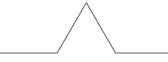
Now what would happen if we repeated this Koch pattern again on each of the order 1 segments? We'd get an order 2 Koch fractal.
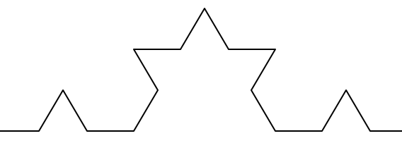
Repeating our pattern again gets us an order 3 Koch fractal.
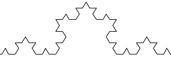
And so on, and so forth. For example this is an order 5 Koch fractal.
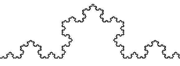
Now let us think about it the other way around. To draw a Koch fractal of order 3, we can simply draw four order 2 Koch fractals. But each of these in turn needs four order 1 Koch fractals, and each of those in turn needs four order 0 fractals. Ultimately, the only drawing that will take place is at order 0. This is very simple to code up in Python:
def koch(t, order, size): """ Makes turtle 't' draw a Koch fractal of 'order' and 'size'. pre: 't' is a Turtle object, ready to draw on some Screen post: A Koch fractal of given 'order' and 'size' has been drawn by turtle 't' on the screen, and the turtle 't' is left facing the same direction. """ if order == 0: # The base case is just a straight line t.forward(size) else: koch(t, order-1, size/3) # Go 1/3 of the way t.left(60) koch(t, order-1, size/3) t.right(120) koch(t, order-1, size/3) t.left(60) koch(t, order-1, size/3) "Of course, to actually run the code above we still need to" "add the necessary instructions to set up the turtle graphics:" import turtle window = turtle.Screen() t = turtle.Turtle() t.speed(0) t.penup() t.forward(-150) t.pendown() koch(t,5,300) # <- Here is the actual call to the koch function ! window.mainloop()
The key thing that is new here is that as long as order is not zero, koch calls itself recursively to get its job done.
Rereading the above code of the koch function, we observe that it contains a quite repetitive pattern. (Do you see it?) Not quite fond of duplicated code, we will try to tighten up the code a bit to get rid of this repetition. First of all, remember that turning right by 120 degrees is the same as turning left by -120 degrees. So with a bit of clever rearrangement, we can use a single loop to make the four recursive calls to the koch function in the else-branch.
def koch(t, order, size): if order == 0: t.forward(size) else: for angle in [60, -120, 60, 0]: koch(t, order-1, size/3) t.left(angle)
The final turn is 0 degrees, so it has no effect. But it has allowed us to find a pattern and reduce seven lines of code to three, which will make things easier for our next observations.
Recursion, the high-level view
One way to think about this is to convince yourself that the function works correctly when you call it for an order 0 fractal. Then do a mental leap of faith, saying "I will assume that Python will handle correctly the four recursive level 0 calls for me in the else-branch, so I don't need to think about that detail. So all I need to focus on now is how to draw an order 1 fractal assuming that the order 0 one is already working."
You're practicing mental abstraction --- ignoring the subproblem while you solve the big problem.
If this mode of thinking works (and you should practice it!), then take it to the next level. Aha! now can I see that it will work when called for order 2 under the assumption that it is already working for level 1.
And, in general, if I can assume the order n-1 case works, can I just solve the level n problem?
Students of mathematics who have played with proofs of induction should see some very strong similarities here.
Recursion, the low-level operational view
Another way of trying to understand recursion is to get rid of it! If we had separate functions to draw a level 3 fractal, a level 2 fractal, a level 1 fractal and a level 0 fractal, we could simplify the above code, quite mechanically, to a situation where there was no longer any recursion, like this:
def koch_0(t, size): t.forward(size) def koch_1(t, size): for angle in [60, -120, 60, 0]: koch_0(t, size/3) t.left(angle) def koch_2(t, size): for angle in [60, -120, 60, 0]: koch_1(t, size/3) t.left(angle) def koch_3(t, size): for angle in [60, -120, 60, 0]: koch_2(t, size/3) t.left(angle)
This trick of "unfolding" the recursion gives us an operational view of what happens. You can trace the program into koch_3, and from there, into koch_2, and then into koch_1, etc., all the way down the different layers of the recursion.
This might be a useful hint to build your understanding. The mental goal is, however, to be able to do the abstraction!
Recursive data structures
All of the Python data types we have seen can be grouped inside lists and tuples in a variety of ways. Lists and tuples can also be nested, providing many possibilities for organizing data. The organization of data for the purpose of making it easier to use is called a data structure.
Suppose it is election time and that we are helping to count votes as they come in. Votes arriving from individual districts, cities, agglomerations and provinces are sometimes reported as a sum total of votes and sometimes as a list of subtotals of votes. After considering how best to store this incoming data, we decide to use a nested number list, which we define as follows:
A nested number list is a list whose elements are either:
- numbers
- nested number lists
Notice how in the above definition, the term nested number list is used to define itself. Recursive definitions like this are quite common in mathematics and computer science. They provide a concise and powerful way to describe recursive data structures that are partially composed of smaller and simpler instances of themselves. The definition is not circular, nor infinite, since at some point we will reach a list that does not have any lists as elements.
Now suppose our job is to write a function that will sum all of the values in a nested number list. Python has a built-in function which finds the sum of a sequence of numbers:
>>> sum([1, 2, 8]) 11
For our nested number list, however, sum will not work:
>>> sum([1, 2, [11, 13], 8]) Traceback (most recent call last): File "<pyshell>", line 1, in <module> TypeError: unsupported operand type(s) for +: 'int' and 'list'
The problem is that the third element of this list, [11, 13], is itself a list, so it cannot just be added to 1, 2, and 8.
Processing recursive number lists
To sum all the numbers in our recursive nested number list we need to traverse the list, visiting each of the elements within its nested structure, adding any numeric elements to our sum, and recursively repeating the summing process with any elements which are themselves sub-lists.
Thanks to recursion, the Python code needed to sum the values of a nested number list is surprisingly short:
def r_sum(nested_num_list): """ Computes the sum of all values in a recursively nested structure of lists. pre: 'nested_num_list' is a nested number list, i.e., a list whose elements are either numbers or again nested number lists. post: returns 0 for empty lists or the sum of all encountered values, at any level of nesting, for nested number lists. """ tot = 0 for element in nested_num_list: if isinstance(element,list): tot += r_sum(element) else: tot += element return tot
>>> r_sum([1, 2, [11, 13], 8]) 35
The body of r_sum consists mainly of a for loop that traverses nested_num_list. If element is a numerical value (the else branch), it is simply added to tot. If element is a list (which is checked with the type check isinstance(element,list)), then r_sum is called again, with the element as an argument. The statement inside the function definition in which the function calls itself is known as the recursive call.
The example above has a base case (the else branch) which does not lead to a recursive call: the case where the element is not a (sub-) list. Without a base case, you'll have infinite recursion, and your program will not work.
Recursion is truly one of the most beautiful and elegant tools in computer science.
A slightly more complicated problem is finding the largest value in a nested number list:
def r_max(nxs): """ Finds the maximum value in a recursively nested structure of lists. pre: 'nxs' is a nested number list, i.e., a list whose elements are either numbers or again nested number lists. No lists or sublists are empty. post: returns the maximum value of all encountered values in this nested structure of lists. """ largest = None first_time = True for e in nxs: if isinstance(e,list): val = r_max(e) else: val = e if first_time or val > largest: largest = val first_time = False return largest test(r_max([2, 9, [1, 13], 8, 6]) == 13) test(r_max([2, [[100, 7], 90], [1, 13], 8, 6]) == 100) test(r_max([[[13, 7], 90], 2, [1, 100], 8, 6]) == 100) test(r_max(["joe", ["sam", "ben"]]) == "sam")
We included some tests to provide examples of r_max at work. (All these assertions should succeed. Figure out for yourself what would happen if the list or one of its nested sublists would be empty.)
The added twist to this problem is finding a value for initializing largest. We can't just use nxs[0], since that could be either an element or a list. To solve this problem (at every recursive call) we set a Boolean flag first_time to True (at line 11). When we've found the value of interest (at line 17), we check to see whether this is the initializing (first) value for largest, or a value that could potentially change largest.
Again here we have a base case at line 15. If we don't supply a base case, Python stops after reaching a maximum recursion depth and returns a runtime error. See how this happens, by running this little script which we will call infinite_recursion.py:
def recursion_depth(number): print("{0}, ".format(number), end="") recursion_depth(number + 1) recursion_depth(0)
After watching the messages flash by, you will be presented with the end of a long traceback that ends with a message like the following:
RecursionError: maximum recursion depth exceeded while calling a Python object
We would certainly never want something like this to happen to a user of one of our programs, so it is good programming practice to write error handling code that could handle such errors when they arise.
Fibonacci numbers
The famous Fibonacci sequence 0, 1, 1, 2, 3, 5, 8, 13, 21, 34, 55, 89, 144, ... [FibonacciNumber] was devised by Fibonacci (1170-1250), who used this to model the breeding of (pairs) of rabbits. If, in generation 8 you had 21 pairs in total, of which 13 were adults, then next generation the adults will all have bred new children, and the previous children will have grown up to become adults. So in generation 9 you'll have 13+21=34, of which 21 are adults.
This model to explain rabbit breeding made the simplifying assumption that rabbits never died. Scientists often make (over-)simplifying assumptions and restrictions to make some headway with the problem.
If we number the terms of the sequence from 0, we can describe each term recursively as the sum of the previous two terms:
fib(0) = 0 fib(1) = 1 fib(n) = fib(n-1) + fib(n-2) for n >= 2
This translates very directly into some Python:
def fib(n): """ Computes numbers in the Fibonacci sequence 0, 1, 1, 2, 3, 5, 8, 13, 21, ... pre: 'n' is natural number (an integer >= 0) post: returns the n-th Fibonacci number, where fib(0) = 0 and fib(1) = 1 and any other Fibonacci number is defined as the sum of the previous 2 Fibonacci numbers, for example: fib(2) = fib(0) + fib(1) = 0 + 1 = 1 """ if n <= 1: return n t = fib(n-1) + fib(n-2) return t test(fib(0) == 0) test(fib(1) == 1) test(fib(2) == 1) test(fib(3) == 2) test(fib(4) == 3) test(fib(5) == 5) test(fib(6) == 8) test(fib(7) == 13) test(fib(8) == 21) test(fib(9) == 34) test(fib(10) == 55) test(fib(11) == 89) test(fib(12) == 144)
This is a particularly inefficient algorithm. One particular way of fixing this inefficiency, which we will leave as an exercise for now, is to make use of dictionaries to remember (or memoize) previously calculated values of the function so that they don't need to be recalculated over and over again.
import time from time import process_time t0 = process_time() n = 35 result = fib(n) t1 = process_time() print("fib({0}) = {1}, ({2:.2f} secs)".format(n, result, t1-t0))
We get the correct result, but an exploding amount of work!
fib(35) = 9227465, (4.51 secs)
Memoization
If you play around a bit with the fib function from the previous section, you will notice that the bigger the argument you provide, the longer the function takes to run. Furthermore, the run time increases very quickly. On one of our machines, fib(20) finishes instantly, fib(30) takes about a second, and fib(40) takes roughly forever.
To understand why, consider this call graph for fib with n = 4:
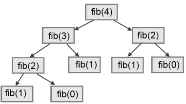
A call graph shows some function frames (instances when the function has been invoked), with lines connecting each frame to the frames of the functions it calls. At the top of the graph, fib with n = 4 calls fib with n = 3 and n = 2. In turn, fib with n = 3 calls fib with n = 2 and n = 1. And so on.
Count how many times fib(0) and fib(1) are called. This is an inefficient solution to the problem, and it gets far worse as the argument gets bigger.
A good solution is to keep track of values that have already been computed by storing them in a dictionary. A previously computed value that is stored for later use is called a memo. Here is an implementation of fib using memos:
alreadyknown = {0: 0, 1: 1} def fib(n): if n not in alreadyknown: new_value = fib(n-1) + fib(n-2) alreadyknown[n] = new_value return alreadyknown[n]
The dictionary named alreadyknown keeps track of the Fibonacci numbers we already know. We start with only two pairs: 0 maps to 1; and 1 maps to 1.
Whenever fib is called, it checks the dictionary to determine if it contains the result. If it's there, the function can return immediately without making any more recursive calls. If not, it has to compute the new value. The new value is added to the dictionary before the function returns.
Using this version of fib, our machines can compute fib(100) in an eyeblink.
>>> fib(100) 354224848179261915075
Example with recursive directories and files
The following program lists the contents of a directory and all its subdirectories. Notice how a recursive function print_files is used to recursively walk through the recursively nested directory structure.
import os def get_dirlist(path): """ Produces the list of all files in a given directory. pre: 'path' is a string describing a valid path to a directory in the operating system. post: Returns a sorted list of the names of all entries (files or directories) encountered in the directory with that path. This returns just the names, not the full path to the names. Directories nested in this directory are not recursively explored. """ dirlist = os.listdir(path) dirlist.sort() return dirlist def print_files(path, prefix = ""): """ Prints the recursive listing of all contents in a given directory. pre: 'path' is a string describing a valid path to a directory in the operating system. post: Prints the path and the names of all entries (files or directories contained in it). Nested directories are visited recursively. For every entry, the nesting level is indicated by vertical bars. Entries directly contained in the path are preceded by one bar, entries at nesting level 2 by two bars, and so on. """ if prefix == "": # Detect outermost call, print a heading print("Folder listing for", path) prefix = "| " dirlist = get_dirlist(path) for f in dirlist: print(prefix+f) # Print the line fullname = os.path.join(path, f) # Turn name into full pathname if os.path.isdir(fullname): # If a directory, recurse. print_files(fullname, prefix + "| ")
Calling the function print_files with some initial path or folder name will produce an output similar to this:
print_files("c:\python31\Lib\site-packages\pygame\examples")
Folder listing for c:\python31\Lib\site-packages\pygame\examples
| __init__.py
| aacircle.py
| aliens.py
| arraydemo.py
| blend_fill.py
| blit_blends.py
| camera.py
| chimp.py
| cursors.py
| data
| | alien1.png
| | alien2.png
| | alien3.png
...
Glossary
- base case
- A branch of the conditional statement in a recursive function that does not give rise to further recursive calls.
- infinite recursion
- A function that calls itself recursively without ever reaching any base case. Eventually, infinite recursion causes a runtime error.
- recursion
- The process of calling a function that is already executing.
- recursive call
- The statement that calls an already executing function. Recursion can also be indirect --- function f can call g which calls h, and h could make a call back to f --- or mutual --- function f calls g and g makes a call back to f.
- recursive definition
- A definition which defines something in terms of itself. To be useful it must include base cases which are not recursive. In this way it differs from a circular definition. Recursive definitions often provide an elegant way to express complex data structures, like a directory that can contain other directories, or a menu that can contain other menus.
References
| [ThinkCS] | How To Think Like a Computer Scientist --- Learning with Python 3 |
| [Fractal] | https://en.wikipedia.org/wiki/Fractal |
| [FibonacciNumber] | https://en.wikipedia.org/wiki/Fibonacci_number |
Higher-Order Functions
Source: This section is heavily based on Section 1.6 of [SICP]. It does not appear in [ThinkCS].
We have seen before that functions are abstractions that describe compound operations independent of the particular values of their arguments. For example, when defining a function square,
def square(x): return x * x
we are not talking about the square of a particular number, but rather about a method for obtaining the square of any number x. Of course we could get along without ever defining this function, by always writing expressions such as:
>>> 3 * 3 9 >>> 5 * 5 25
and never mentioning square explicitly. This practice would suffice for simple computations like square, but would become arduous for more complex examples. In general, lacking function definition would put us at the disadvantage of forcing us to work always at the level of the particular operations that happen to be primitives in the language (multiplication, in this case) rather than in terms of higher-level operations. Our programs would be able to compute squares, but our language would lack the ability to express the concept of squaring. One of the things we demand from a powerful programming language is the ability to build abstractions by assigning names to common patterns and then to work in terms of these abstractions directly. Functions provide this ability.
As we will see in the following examples, there are common programming patterns that recur in code, but are used with a number of different functions. These patterns can also be abstracted, by giving them names.
To express certain general patterns as named concepts, we will need to construct functions that can accept other functions as arguments or that return functions as values. Such functions that manipulate functions are called higher-order functions. This section shows how higher-order functions can serve as powerful abstraction mechanisms, vastly increasing the expressive power of our language.
Functions as Arguments
Consider the following three functions, which all compute summations. The first, sum_naturals, computes the sum of natural numbers up to n:
def sum_naturals(n): total, k = 0, 1 while k <= n: total, k = total + k, k + 1 return total
>>> sum_naturals(100) 5050
The second, sum_cubes, computes the sum of the cubes of natural numbers up to n.
def sum_cubes(n): total, k = 0, 1 while k <= n: total, k = total + pow(k, 3), k + 1 return total
>>> sum_cubes(100) 25502500
The third, pi_sum, computes the sum of terms in the series
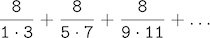
which converges to pi, though very slowly.
def pi_sum(n): total, k = 0, 1 while k <= n: total, k = total + 8 / (k * (k + 2)), k + 4 return total
>>> pi_sum(100) 3.121594652591009
These three functions clearly share a common underlying pattern. They are for the most part identical, differing only in their name, the function of k used to compute the term to be added, and the function that provides the next value of k. We could generate each of the functions by filling in the slots <name>, <term> and <next> in the following template:
def <name>(n): total, k = 0, 1 while k <= n: total, k = total + <term>(k), <next>(k) return total
The presence of such a common pattern is strong evidence that there is a useful abstraction waiting to be brought to the surface. Each of these functions is a summation of terms. As program designers, we would like our language to be powerful enough so that we can write a function that expresses the concept of summation itself rather than only functions that compute particular sums. We can do so readily in Python by taking the common template shown above and transforming the "slots" into formal parameters of a more general summation function.
def summation(n, term, next): total, k = 0, 1 while k <= n: total, k = total + term(k), next(k) return total
Notice that summation takes as its arguments the upper bound n together with the functions term and next. We can use summation just as we would any function, and it expresses summations succinctly. For example, we could rewrite our earlier definition of sum_cubes(n) by making use of summation as follows:
def cube(k): return pow(k, 3) def successor(k): return k + 1 def sum_cubes(n): return summation(n, cube, successor)
>>> sum_cubes(3) 36
Using as term function an identity function that returns its argument, we can also sum integers.
def identity(k): return k def sum_naturals(n): return summation(n, identity, successor)
>>> sum_naturals(10) 55
We can even define pi_sum piece by piece, using our summation abstraction to combine components.
def pi_term(k): denominator = k * (k + 2) return 8 / denominator def pi_next(k): return k + 4 def pi_sum(n): return summation(n, pi_term, pi_next)
>>> pi_sum(1e6) 3.1415906535898936
Functions as General Methods of Computation
We introduced user-defined functions as a mechanism for abstracting patterns of numerical operations so as to make them independent of the particular numbers involved. With higher-order functions, we begin to see a more powerful kind of abstraction: some functions express general methods of computation, independent of the particular functions they call.
To illustrate this mechanism, in this subsection we will build an abstraction for a general method of computation known as iterative improvement, and use it to compute the golden ratio [GoldenRatio]. An iterative improvement algorithm begins with a guess of a solution to an equation. It then repeatedly applies an update function to improve that guess, and applies a test to check whether the current guess is "close enough" to the expected solution to be considered correct.
def iter_improve(update, test, guess=1): while not test(guess): guess = update(guess) return guess
The test function typically checks whether two functions, f and g, are near to each other for a particular value of guess. Testing whether f(x) is near to g(x) is again a general method of computation.
def near(x, f, g): return approx_eq(f(x), g(x))
A common way to test for approximate equality in programs is to compare the absolute value of the difference between numbers to a small tolerance value.
def approx_eq(x, y, tolerance=1e-5): return abs(x - y) < tolerance
The golden ratio, often called phi, is a number that appears frequently in nature, art, and architecture. It can be found by applying the formula phi = 1 + 1/phi recursively until phi^2 = phi + 1. [GoldenRatio] In other words, we can compute the golden ratio via iter_improve using the golden_update function phi = 1 + 1/phi, and it converges when its successor phi + 1 is equal to its square phi^2.
def golden_update(guess): return 1 + 1/guess def golden_test(guess): return near(guess, square, successor)
Calling iter_improve with the arguments golden_update and golden_test will compute an approximation to the golden ratio.
>>> approx_phi = iter_improve(golden_update, golden_test) >>> approx_phi 1.6180371352785146
This extended worked-out example illustrates two related big ideas in computer science. First, naming and functions allow us to abstract away a vast amount of complexity. While each individual function definition was quite trivial, the computational process set in motion is quite intricate. Second, it is only by virtue of the fact that we have an extremely general evaluation procedure that small components can be composed into complex processes.

To conclude this example, it would be good if we could check the correctness of our new general method iter_improve. The computation of the golden ratio provide such a test, because we used iter_improve to compute the golden ratio, so we only need to compare that computed value with its exact closed-form solution phi = (1 + square_root(5))/2. [GoldenRatio]
def square_root(x): return pow(x, 1/2) phi = (1 + square_root(5))/2 # => 1.618033988749895 def near_test(): assert near(phi, square, successor), 'phi * phi is not near phi + 1' def iter_improve_test(): approx_phi = iter_improve(golden_update, golden_test) assert approx_eq(phi, approx_phi), 'phi differs from its approximation'
Nested Function Definitions
The worked-out example above demonstrates how the ability to pass functions as arguments significantly enhances the expressive power of a programming language. Each general concept or equation maps onto its own short function. One negative consequence of this approach to programming is that the global namespace becomes cluttered with names of many small auxiliary functions. Another problem is that we are constrained by particular function signatures: the update argument to iter_improve must be a function that takes exactly one argument. In Python, nested function definitions address both of these problems.
Let's consider a new problem: computing the square root of a number. It can be shown that repeated application of the following update function converges to the square root of x:
def average(x, y): return (x + y)/2 def sqrt_update(guess, x): return average(guess, x/guess)
This two-argument update function is incompatible with iter_improve however, since it takes two arguments instead of one. Furthermore, it is just an intermediate auxiliary function: we really only care about taking square roots and don't necessarily want others to see or use this auxiliary function. The solution to both of these issues is to place function definitions inside the body of other definitions.
def square_root(x): def update(g): return average(g, x/g) def approx_eq(x, y, tolerance=1e-5): return abs(x - y) < tolerance def test(guess): return approx_eq(square(guess), x) return iter_improve(update, test)
>>> square_root(81) 9.000000000007091
Like local variable assignment, local function definitions only affect the body of the function in which they are defined. These local functions will only be visible and usable while square_root is being evaluated. Moreover, these local def statements won't even get evaluated until square_root is called. Their definition is part of the evaluation of square_root .
Lexical scope. Locally defined functions have access to the name bindings in the local scope in which they are defined. In this example, the nested function test can make use of the nested function approx_eq because it is defined in the same scope. Similarly, the expression iter_improve(update, test) in the body of square_root can make use of the locally defined functions update and test . Furthermore, the nested functions update and test can refer to the name x, which is a formal parameter of its enclosing function square_root . (Upon calling square_root , this formal parameter will be bound to the actual value passed as parameter when calling the function.) This discipline of sharing names among nested definitions is called lexical scoping: all inner functions have access to the names in the environment where they are defined (not where they are called).
Nested scopes. Whenever a name cannot be found in a local scope, it will be looked up in the surrounding scope. For example, in the function definition of update nested inside the definition of square_root , a function named average is being referred to. Upon calling this update function, it will first look for this name in its own local scope (it could have been that average would have been defined as a local function nested inside the definition of update itself). Since it doesn't find any definition of the name average there, it goes to the surrounding scope, that is, the lexical scope in which the update function was defined (the body of the square_root function). Again, there doesn't seem to be any function named average defined there (there are only the functions approx_eq and test defined there). Again, the name lookup goes one level up, reaching the global environment in which square_root itself was initially defined. Luckily a definition of the average function is finally found there.
Shadowing. As explained above, names are always resolved from innermost to outermost scopes. This implies that, if a more local scope defines a variable or function with the same name as one that already exists in a surrounding scope, it hides or shadows that variable, so that locally only the innermost value assigned to that name will be visible. This is for example the case for the variable named x used inside the body of the nested function approx_eq . The expression return abs(x - y) < tolerance makes use of a variable named x . When calling the function approx_eq with concrete values for its formal parameters x, y and tolerance , a local environment will be created where these formal parameters will be bound to those concrete values. It is those values of x , y and tolerance that will be used when evaluation the expression return abs(x - y) < tolerance. The value of x visible in the surrounding scope, that is, the value for the formal parameter x of square_root , will be shadowed by the value of x in the more local environment created when evaluating approx_eq.
Let us now illustrate how all this works with a picture. Suppose we evaluate the following expression:
>>> square_root(256) 16.00000000000039
In the global environment, the functions square_root , iter_improve and square are defined. When we evaluate square_root(256) , a new local environment is created that contains a binding of the formal parameter x of the square_root function to the value 256. Furthermore, the square_root function defines three nested functions update, approx_eq and test. These functions definitions are also added to this new local environment (in the picture below, for conciseness, only update is shown). Notice how the local definition of these functions keep a pointer back to the local environment in which they were defined. We will see soon that this is the essence of the mechanism of lexical scoping: all expressions within these inner functions need to have access to the names in the environment where they were defined.
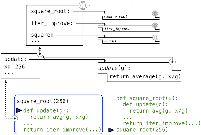
After these nested function definitions, the expression return iter_improve(update, test) in the body of the square_root function needs to be evaluated. The name update, which is passed as an argument to iter_improve , is looked up and resolved to the newly defined function. The same happens for the name test.
With these bindings for update and test , the function call iter_improve(update, test) now gets evaluated. For this evaluation, a new local environment is created where update and test are bound to these functions (again, in the picture below, only update is shown), and where guess is bound to its default value 1. Since iter_improve was defined in the global environment, this local environment points to the global environment, so that it can lookup unresolved names in the environment where the function iter_improve that is being called was originally defined.
Within the body of iter_improve, in the while condition, we must apply the update function to the initial guess of 1. This final application again creates a new local environment for update that contains only a binding of its formal parameter g bound to the value 1.
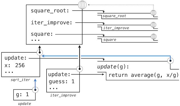
The most crucial part of this evaluation procedure is to find out to what other environment this new local environment should point. This is highlighted by the blue arrows in the diagram. The environment created for the update call, will be scoped within the environment in which update was defined, which can be found by following the blue link back from the update function to its environment of definition (which was the environment created when evaluating square_root(256) and that still contains a binding for x).
In this way, the body of update can resolve a value for x. Hence, we realize two key advantages of lexical scoping in Python.
- The names of a local function do not interfere with names external to the function in which it is defined, because the local function name will be bound in the current local environment in which it is defined, rather than the global environment.
- A local function can access the environment of the enclosing function. This is because the body of the local function is evaluated in an environment that extends the evaluation environment in which it is defined.
The update function thus implicitly carries with it some data: the values referenced in the environment in which it was defined. Because they enclose information in this way, locally defined functions are often called closures.
Functions as Returned Values
We can achieve even more expressive power in our programs by creating functions whose returned values are themselves functions. An important feature of lexically scoped programming languages is that locally defined functions keep their associated environment when they are returned. The following example illustrates the utility of this feature.
With many simple functions defined, function composition is a natural method of combination to include in our programming language. That is, given two functions f(x) and g(x), we might want to define h(x) = f(g(x)). We can define function composition using our existing tools:
def compose1(f, g): def h(x): return f(g(x)) return h
>>> add_one_and_square = compose1(square, successor) >>> add_one_and_square(12) 169
The 1 in compose1 indicates that the composed functions and returned result all take 1 argument. This naming convention isn't enforced by the interpreter; the 1 is just part of the function name.
Lambda Expressions
So far, every time we want to define a new function, we need to give it a name. But for other types of expressions, we don’t need to associate intermediate products with a name. That is, we can compute a*b + c*d without having to name the subexpressions a*b or c*d, or the full expression a*b + c*d. In Python, we can create function values on the fly using lambda expressions, which evaluate to unnamed functions. A lambda expression evaluates to a function that has a single return expression as its body. Assignment and control statements are not allowed.
As opposed to functional programming languages, lambda expressions in Python are quite limited: they are only useful for simple, one-line functions that evaluate and return a single expression. In those special cases where they apply, lambda expressions can be quite expressive, however.
def compose1(f,g): return lambda x: f(g(x))
We can understand the structure of a lambda expression by constructing a corresponding English sentence:
lambda x : f(g(x)) "A function that takes x and returns f(g(x))"
Some programmers find that using unnamed functions from lambda expressions is shorter and more direct. However, compound lambda expressions are notoriously illegible, despite their brevity. The following definition is correct, but some programmers have trouble understanding it quickly.
compose1 = lambda f,g: lambda x: f(g(x))
In general, Python style prefers explicit def statements to lambda expressions, but allows them in cases where a simple function is needed as an argument or return value.
Such stylistic rules are merely guidelines; you can program any way you wish. However, as you write programs, think about the audience of people who might read your program one day. If you can make your program easier to interpret, you will do those people a favor.
The term lambda is a historical accident resulting from the incompatibility of written mathematical notation and the constraints of early type-setting systems.
It may seem perverse to use lambda to introduce a procedure/function. The notation goes back to Alonzo Church, who in the 1930's started with a "hat" symbol; he wrote the square function as "ŷ . y × y". But frustrated typographers moved the hat to the left of the parameter and changed it to a capital lambda: "Λy . y × y"; from there the capital lambda was changed to lowercase, and now we see "λy . y × y" in math books and (lambda (y) ( y y)) in Lisp.* ---Peter Norvig (norvig.com/lispy2.html)
Despite their unusual etymology, lambda expressions and the corresponding formal language for function application, the lambda calculus, are fundamental computer science concepts shared far beyond the Python programming community. You will very likely encounter it in other programming languages or other computer science courses.
Example: Newton's Method
This final extended example shows how function values, local definitions, and lambda expressions can work together to express general ideas concisely.
Newton's method is a classic iterative approach to finding the arguments x for which a single-argument mathematical function f(x) yields a return value of 0. In other words, the values of x for which that function f cuts the x-axis (f(x) = 0). These values are called the roots of that function. Finding a root of a single-argument mathematical function is often equivalent to solving a related math problem. For example:
The square root of 16 is the value x such that: square(x) - 16 = 0 .
The logarithm with base 2 of 32 is the value x such that: pow(2, x) - 32 = 0 (i.e., the exponent x to which we would raise 2 to get 32).
Thus, a general method for finding the roots of a function would also provide us an algorithm to compute square roots and logarithms. Moreover, the functions for which we want to compute roots contain simpler operations (multiplication and exponentiation) than the original function we want to compute (square root and logarithm).
A comment before we proceed: it is easy to take for granted the fact that we know how to compute square roots and logarithms. Not just Python, but your phone, your pocket calculator, and perhaps even your watch can do so for you. However, part of learning computer science is understanding how quantities like these can be computed, and the general approach presented here is applicable to solving a large class of equations beyond those built into Python.
Before even beginning to understand Newton's method, we can start programming; this is the power of functional abstractions. We simply translate our previous statements into code.
def square_root(a): return find_root(lambda x: square(x) - a) def logarithm(a, base=2): return find_root(lambda x: pow(base, x) - a)
Of course, we cannot apply any of these functions yet until we define find_root, and so we need to understand how Newton's method works.
Like the algorithm we saw before, Newton's method is also an iterative improvement algorithm. It improves a guess of the root for any function that is differentiable (in the mathematical sense). Notice that both of our functions of interest change smoothly; graphing x versus f(x) for
f(x) = square(x) - 16 (light curve) f(x) = pow(2, x) - 32 (dark curve)
on a 2-dimensional plane shows that both functions produce a smooth curve without kinks that crosses the x-axis (f(x)=0) at the appropriate point.
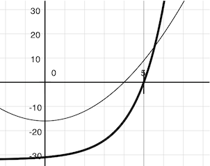
Because they are smooth (differentiable), these curves can be approximated by a line at any point. Newton's method follows these linear approximations to find function roots.
Imagine a line through the point (x, f(x)) that has the same slope as the curve for function f(x) at that point. Such a line is called the tangent, and its slope is called the derivative of f at x.
This line's slope is the ratio of the change in function value to the change in function argument. Hence, translating x by f(x) divided by the slope will give the argument value at which this tangent line touches 0.
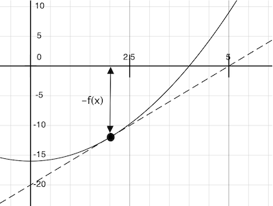
Our newton_update function expresses the computational process of following this tangent line to 0. We approximate the derivative of the function by computing its slope over a very small interval.
def approx_derivative(f, x, delta=1e-5): df = f(x + delta) - f(x) return df/delta def newton_update(f): def update(x): return x - f(x) / approx_derivative(f, x) return update
Finally, we can define the find_root function in terms of newton_update, our iterative improvement algorithm, and a test to see if f(x) is near 0. We supply a larger initial guess to improve the performance for logarithm.
def find_root(f, initial_guess=10): def test(x): return approx_eq(f(x), 0) return iter_improve(newton_update(f), test, initial_guess)
>>> square_root(16) 4.000000000026422 >>> logarithm(32, 2) 5.000000094858201
And to verify that these values are correct, you can test:
>>> square(square_root(16)) 16.00000000021138 >>> pow(2,logarithm(32, 2)) 32.0000021040223
As you experiment with Newton's method, be aware that it will not always converge. The initial guess of iter_improve must be sufficiently close to the root, and various conditions about the function must be met. Despite this shortcoming, Newton's method is a powerful general computational method for solving differentiable equations. In fact, very fast algorithms for logarithms and large integer division employ variants of the technique.
Abstractions and First-Class Functions
We began this section with the observation that user-defined functions are a crucial abstraction mechanism, because they permit us to express general methods of computing as explicit elements in our programming language. Now we've seen how higher-order functions permit us to manipulate these general methods to create further abstractions.
As programmers, we should be alert to opportunities to identify the underlying abstractions in our programs, to build upon them, and generalize them to create more powerful abstractions. This is not to say that one should always write programs in the most abstract way possible; expert programmers know how to choose the level of abstraction appropriate to their task. But it is important to be able to think in terms of these abstractions, so that we can be ready to apply them in new contexts. The significance of higher-order functions is that they enable us to represent these abstractions explicitly as elements in our programming language, so that they can be handled just like other computational elements.
In general, programming languages impose restrictions on the ways in which computational elements can be manipulated. Elements with the fewest restrictions are said to have first-class status. Some of the "rights and privileges" of first-class language elements are:
- They may be bound to names.
- They may be passed as arguments to functions.
- They may be returned as the results of functions.
- They may be included in data structures.
Python awards functions full first-class status, and the resulting gain in expressive power is enormous. Control structures, on the other hand, do not: you cannot pass if to a function the way you can sum.
Function Decorators
Python provides special syntax to apply higher-order functions as part of executing a def statement, called a decorator. Perhaps the most common example is a trace.
def trace1(f): def wrapped(x): print('-> ', f, '(', x, ')') return f(x) return wrapped @trace1 def triple(x): return 3 * x
>>> triple(12) -> <function triple at 0x102a39848> ( 12 ) 36
In this example, a higher-order function trace1 is defined, which returns a function that precedes a call to its argument with a print statement that outputs the argument. The def statement for triple has an annototation, @trace1, which affects the execution rule for def. As usual, the function triple is created. However, the name triple is not bound to this function. Instead, the name triple is bound to the returned function value of calling trace1 on the newly defined triple function. In fact, in code this decorator is equivalent to:
def triple(x): return 3 * x triple = trace1(triple)
If you want, try and apply the @trace1 annotation to the Fibonacci function fib(n) before calling it with some value of n, to observe to how many recursive calls it leads.
@trace1 def fib(n): if n <= 1: return n return fib(n-1) + fib(n-2) fib(10)
>>> fib(5) -> <function fib at 0x104147d90> ( 5 ) -> <function fib at 0x104147d90> ( 4 ) -> <function fib at 0x104147d90> ( 3 ) -> <function fib at 0x104147d90> ( 2 ) -> <function fib at 0x104147d90> ( 1 ) -> <function fib at 0x104147d90> ( 0 ) -> <function fib at 0x104147d90> ( 1 ) -> <function fib at 0x104147d90> ( 2 ) -> <function fib at 0x104147d90> ( 1 ) -> <function fib at 0x104147d90> ( 0 ) -> <function fib at 0x104147d90> ( 3 ) -> <function fib at 0x104147d90> ( 2 ) -> <function fib at 0x104147d90> ( 1 ) -> <function fib at 0x104147d90> ( 0 ) -> <function fib at 0x104147d90> ( 1 ) 5
Decorators can be used for tracing, for selecting which functions to call when a program is run from the command line, and many other things.
Extra for experts. The actual rule is that the decorator symbol @ may be followed by an expression (@trace1 is just a simple expression consisting of a single name). Any expression producing a suitable value is allowed. For example, with a suitable definition, you could define a decorator check_range so that decorating a function definition with @check_range(1, 10) would cause the function's results to be checked to make sure they are integers between 1 and 10. The call check_range(1,10) would return a function that would then be applied to the newly defined function before it is bound to the name in the def statement.
Glossary
- higher-order functions
- Higher-order functions are functions that can accept other functions as arguments or that return functions as values.
- general methods of computation
- Higher-order functions can serve as powerful abstraction mechanisms to express general methods of computation, independent of the particular functions they call. These higher-order functions can then be supplied with particular functions to produce more specific computations. For example, a higher-order function that expresses the high-level computational process of iterative improvement, could be customized, by providing the right functions as arguments, into a method for computing an approximation of the golden ratio.
- nested functions
- Nested function definitions are functions that are defined locally in the body of another function definition. Nested function definitions have two main advantages. Firstly, because the functions are defined locally, they don't clutter the global namespace with the names of many small auxiliary functions. Secondly, since the functions are scoped within the body of another function, they have access to all parameters and variables declared locally inside that other function. Because of that, those nested functions often require less parameters than if they would have been defined globally.
- lexical scope
- The discipline of sharing names among nested definitions is called lexical scoping: all nested function definitions have access to the names visible in their environment of definition (as opposed to the environment where they were called).
- nested scope
- Since function definitions can be nested inside other function definitions, which can again be nested inside other function definitions, we can have multiple layers of nested lexical scopes. In such cases, name resolution (i.e., the process of looking up names for variables or functions) will proceed layer by layer from the inner-most scope where a function was defined until it eventually reaches the outermost global namespace.
- shadowing
- Related to nested scopes, shadowing refers to a situation where two (variable or function) names exist within scopes that overlap. Whenever that happens, the name with the outermost scope is hidden because the variable with the more nested scope overrides it. The outermost variable is said to be shadowed by the innermost one.
- function as returned value
- In Python, just like it is possible to create functions that take other functions are arguments, it is possible to write functions whose returned values are themselves functions.
- lambda expression
- Lambda expressions are a way to define new functions, without needing to give them a name. A lambda expression evaluates to a function that has a single return expression as its body. Lambda expressions in Python are quite limited: they are only useful for simple, one-line functions that evaluate and return a single expression. Assignment and control statements are not allowed.
- first-class functions
- In general, programming languages impose restrictions on how certain language elements can be manipulated. Elements with the fewest restrictions are said to have first-class status. Some of the "rights and privileges" of first-class language element are that they can be bound to names, be passed as arguments to functions, be returned as the results of functions and that they may be included in data structures. Since all this is the case for functions in Python, functions are first-class elements in Python.
- function decorators
- By definition, a function decorator is a function that takes another function and extends the behavior of the latter function without explicitly modifying it. Function decorators provide a simple syntax for calling higher-order functions, by simply annotating the definition of a function with the higher-order function that needs to be applied to it upon calling that function.
References
| [SICP] | SICP in Python. This book is derived from the classic textbook "Structure and Interpretation of Computer Programs" by Abelson, Sussman, and Sussman. John Denero originally modified it for Python in 2011. It is licensed under the Creative Commons Attribution-ShareAlike 3.0 license. |
| [ThinkCS] | How To Think Like a Computer Scientist --- Learning with Python 3 |
| [GoldenRatio] | (1, 2, 3) https://en.wikipedia.org/wiki/Golden_ratio |